Physical Problem for Integration: Computer Engineering

Physical Problem for Integration:Computer Engineering 07.00D.1

Chapter 07.00D

Physical Problem for Integration

Computer Engineering

Problem

Human vision has the remarkable ability to infer 3D shapes from 2D images. When we look at 2D photographs or TV we do not see them as 2D shapes, rather as 3D entities with surfaces and volumes. Perception research has unraveled many of the cues that are used by us. The intriguing question is: can we replicate some of these abilities on a computer? To this end, in this assignment we are going to look at one way to engineer a solution to the 3D shape from 2D images problem. Apart from the pure fun of solving a new problem, there are many practical applications of this technology such as in automated inspection of machine parts, inference of obstructing surfaces for robot navigation, and even in robot-assisted surgery.

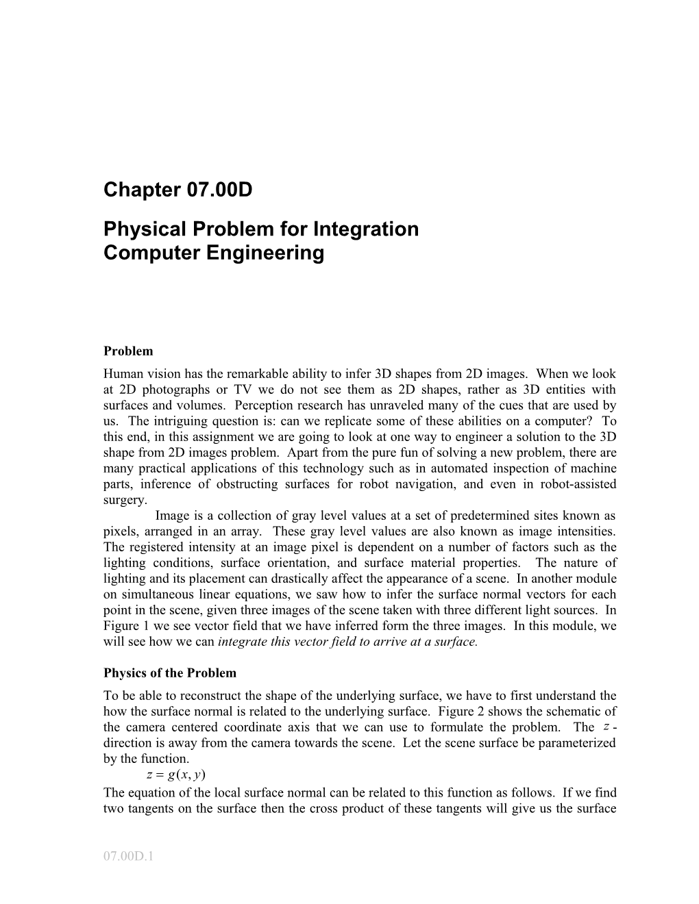
Image is a collection of gray level values at a set of predetermined sites known as pixels, arranged in an array. These gray level values are also known as image intensities. The registered intensity at an image pixel is dependent on a number of factors such as the lighting conditions, surface orientation, and surface material properties. The nature of lighting and its placement can drastically affect the appearance of a scene. In another module on simultaneous linear equations, we saw how to infer the surface normal vectors for each point in the scene, given three images of the scene taken with three different light sources. In Figure 1 we see vector field that we have inferred form the three images. In this module, we will see how we can integrate this vector field to arrive at a surface.

Physics of the Problem

To be able to reconstruct the shape of the underlying surface, we have to first understand the how the surface normal is related to the underlying surface. Figure 2 shows the schematic of the camera centered coordinate axis that we can use to formulate the problem. The -direction is away from the camera towards the scene. Let the scene surface be parameterized by the function.

The equation of the local surface normal can be related to this function as follows. If we find two tangents on the surface then the cross product of these tangents will give us the surface normal. Two tangents along the and -directions can easily be specified in terms of the derivatives along these directions. Figure 2 shows the underlying geometry that can be used to arrive at these equations.

and

Figure 2 Relationship between surface tangent at a point to underlying surface equation. On the left is a simplified representation of the imaging geometry. The surface is assumed to be far away from the camera. On the right is a schematic of the local geometry on the scene surface.

The local surface normal, , will be along the direction of the cross product of and .

Note that there is 1800 ambiguity in the specification of the surface normal. We need the negative sign because we want the surface normal to be oriented towards the camera and the -axis is pointed away from the camera. Also, note that the cross product gives as a vector along the surface normal. We have to normalize the vector to arrive at the surface normal. For notational ease let

and

Then,

We see that the surface normal can be expressed in terms of the derivatives of the underlying surface. From this equation, we can express the local surface derivatives in terms of ratios of the surface normal components.

and

The black lines denote possible paths over which the x-partial derivative can be integrated. And, the purple lines denote possible paths to integrate the y-partial derivative. The paths are shown overlaid on the input vector field representing the partial derivatives of the surface along x and y directions.

Solution

We arrive at the final surface equation by integration these partial derivatives. Since we have a 2D field, we can perform the integration along many paths. The simplest paths are along the (or ) axis.

or

One could also start from the right edge of the image and integrate the partial derivative with respect to towards the left edge, or start from the bottom of the image and integrate the -partial derivative towards the top. These directions are depicted in Figure 3. The equivalent integrals are as follows. The image is assumed to N pixels by M pixels in size and the negative sign arises because of the direction of the integration.

or

Ideally, all the four integrals should result in the same value, however, for noisy, real world data they will never be the same. One solution is to take the average of these four integrals as the final value. Note that these integrals have to be evaluated for each location in the image to arrive at the full surface.

Worked Out Example

Consider the problem of estimating the surface height along the line passing through the center of the sphere in Figure 1. Figure 4 (a) shows the input estimates for the partial derivatives along the x direction, for the sphere along this line. The raw data for this plot is given below.

This data needs to be numerically integrated to arrive at height values. Figure 4 (b) shows the plot of the surface height, as computed by integrating starting from left and from right. We used the trapezoidal integration method. Notice the small discrepancy, which is due to real world data noise. The overall shape does look circular, which should serve as a sanity check on the calculations.

Figure 4(a)

Figure 4(b)

Figure 4(a) The plot of the estimates for the partial derivatives along the x direction, for the sphere along a horizontal line passing through the middle of the sphere. Figure 4(b) Plot of the integrated value at each point along the horizontal. The blue plot corresponds to integrating from left to right and the red plot corresponds to integrating from right to left.

If we repeat the above process along the vertical direction (along image columns), then we will arrive at two more estimates for the middle point of the sphere, which can be averaged to arrive at one estimate. If we repeat this for each point on the sphere, not just the middle, then we will arrive at the surface representation for the full sphere. Figure 5 shows the averaged estimate of the sphere as estimated from the input vector field. Note the spherical nature of the final estimate.

QUESTIONS

1. Write code to recover the surface height at each point in the image given the vector field.
2. For any point on the sphere, specify 25 different paths along which you can integrate.
3. Study how the roughness of the estimated surface changes with number of path integrals that are averaged.