SECOND HOUR EXAM Circle Hour of Class Registered

252y0562 11/9/2005 (Page layout view!)

ECO252 QBA2 Name KEY

SECOND HOUR EXAM Circle Hour of Class Registered

November 9, 2005 MWF2, MWF3, TR12:30, TR3

Show your work! Make Diagrams! Exam is normed on 50 points. Answers without reasons are not usually acceptable.

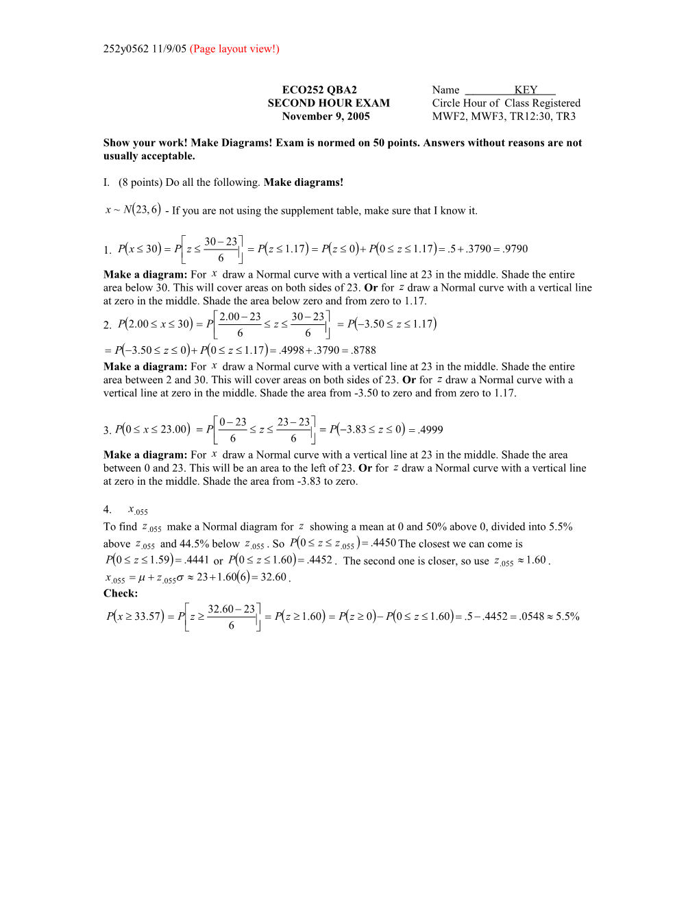
I. (8 points) Do all the following. Make diagrams!

- If you are not using the supplement table, make sure that I know it.

Make a diagram: For draw a Normal curve with a vertical line at 23 in the middle. Shade the entire area below 30. This will cover areas on both sides of 23. Or for draw a Normal curve with a vertical line at zero in the middle. Shade the area below zero and from zero to 1.17.

Make a diagram: For draw a Normal curve with a vertical line at 23 in the middle. Shade the entire area between 2 and 30. This will cover areas on both sides of 23. Or for draw a Normal curve with a vertical line at zero in the middle. Shade the area from -3.50 to zero and from zero to 1.17.

Make a diagram: For draw a Normal curve with a vertical line at 23 in the middle. Shade the area between 0 and 23. This will be an area to the left of 23. Or for draw a Normal curve with a vertical line at zero in the middle. Shade the area from -3.83 to zero.

To find make a Normal diagram for showing a mean at 0 and 50% above 0, divided into 5.5% above and 44.5% below . So The closest we can come is or . The second one is closer, so use . .

Check:

II. (24+ points) Do all the following? (2points each unless noted otherwise).

Computer problem is at the end. Note that some formulas have been squashed by a bug in Word. They should print correctly and will read right if you click on them.

Exhibit 1

The director of the MBA program of a state university wanted to know if a one week orientation would change the proportion among potential incoming students who would perceive the program as being good. Given below is the result from 215 students’ view of the program before and after the orientation.

After the Orientation
Before the Orientation / Good / Not Good / Total
Good / 93 / 37 / 130
Not Good / 71 / 14 / 85
Total / 164 / 51 / 215

Referring to Exhibit 1, which test should she use?

a) -test for difference in proportions

b) Z-test for difference in proportions

c) McNemar test for difference in proportions

d) Wilcoxon rank sum test

ANSWER: c

TYPE: MC DIFFICULTY: Moderate

KEYWORDS: McNemar test, assumption

In Method D6b, the McNemar Test, we compare two proportions taken from the same sample. Assume that two different questions are asked of the same group with the following responses. In this case If we wish to test ,where is the proportion saying ‘yes’ before and is the proportion saying ‘yes’ after, let (The test is valid only if .)

Referring to Exhibit 1, what is the null hypothesis?

Solution: See above.

Referring to Exhibit 1, what is the value of the computed test statistic?

Solution: See above. ANSWER: 3.37 or -3.37

TYPE: PR DIFFICULTY: Moderate

KEYWORD: McNemar test, test statistic

Referring to Exhibit 1, what should be the director’s conclusion?

a) There is sufficient evidence that the proportion of potential incoming students who perceive the program as being good is the same before and after the orientation.

b) There is insufficient evidence that the proportion of potential incoming students who perceive the program as being good is the same before and after the orientation.

c) *There is sufficient evidence that the proportion of potential incoming students who perceive the program as being good is not the same before and after the orientation.

d) There is insufficient evidence that the proportion of potential incoming students who perceive the program as being good is not the same before and after the orientation.

ANSWER: c

TYPE: TF DIFFICULTY: Moderate

KEYWORD: McNemar test, conclusion

. Since .0010 is below , we reject the null hypothesis.

Exhibit 2 (This was Problem D7)

In a study of sleep gotten with a sleeping pill and with a placebo the results were (Keller, Warren, Bartel, 2nd ed. p. 354)

Pill Placebo difference

7.3 6.8 .5

8.5 7.9 .6

6.4 6.0 .4

9.0 8.4 .6

6.9 6.5 .4

We want to see if the means or medians, as appropriate, are different.

Assume these are paired samples from a Normal distribution.

Referring to Exhibit 2, what should be the degrees of freedom for this test?

a) *

d) (Rounded to 7.)

e) Degrees of freedom are irrelevant because we are using a (Mann-Whitney-) Wilcoxon rank sum test.

f) Degrees of freedom are irrelevant because we are using a Wilcoxon signed rank test.

g) We do not have enough information to answer this question. (You must explain what information is missing)

Referring to Exhibit 2, in the formula , we should use the following.

a) *

c) , which is used to compute

d) The standard error is irrelevant because we are using a (Mann-Whitney-) Wilcoxon signed rank test.

e) The standard error is irrelevant because we are using a (Mann-Whitney-) Wilcoxon signed rank test.

f) We do not have enough information to answer this question. (You must explain what information is missing)

Referring to Exhibit 2, assume that the correct alternate hypothesis is , that use of the

formula is correct, that and that there are 27

degrees of freedom (Assume that all of these are correct, even though it is very unlikely!), we should do the following.

a) Reject the null hypothesis only if the significance level is a value below .025

b) Reject the null hypothesis if the significance level is any value below .025

c) Reject the null hypothesis if the significance level is any value above .025

d) Reject the null hypothesis if the significance is any value above .05

e) *Reject the null hypothesis if the significance level is any value above .10

f) None of the above.

Explanation: Note and so that, for a 2-sided test, the p-value is between .05 and .10. If the p-value is below the significance level, reject the null hypothesis.

You are having a part produced in two different machines. is 101 randomly selected data points that represent the length of parts from machine one, is 126 randomly selected data points that represent the length of parts from machine two. You want to test your suspicion that parts from machine one are more variable in length than parts from machine two (This is the same as saying that machine 2 is more reliable than machine 1). Test this suspicion after stating your hypotheses. Your sample means are 25.593 inches for machine 1 and 25.592 for machine 2. Sample standard deviations are 8.379 for machine 1 and 6.964 for machine 2.

Solution:

or . In terms of the variance ratio or , the alternate hypothesis rules, so and .

Since you are comparing variances, use Method D7. Compare the ratio against . This has the F distribution with 100 and 125 degrees of freedom. From the table . Since the computed F is larger than the table F, reject the null hypothesis.

(Extra credit) compute a confidence interval for the ratio of the two variances in the previous problem.

Solution: From the outline . has the F distribution with 100 and 125 degrees of freedom. . . must be between and , probably about 1.46. The interval thus becomes or .

The following problem is an easier version of a problem in the text.

A pet food canning factory produces 8 oz cans of cat food. The manager suspects that the amount of cat food put into the cans by machine 2 is significantly larger than that put in by machine 1. A sample of output is taken with the results below.

a) What are the manager’s null and alternate hypotheses? (1)

b) You will use a test ratio of the form to test the hypothesis. Find (3)

Warning: Be accurate! is roughly the size of .0000175. If you start rounding excessively, your answers will be completely wrong. If you absolutely cannot do this section, say so and use .000175, which is very wrong.

c) Compute the test ratio and find a p-value for your result. (2)

d) If the manager had, instead, suspected that a larger amount was going into cans filled by machine 1, what would the p-value be? (1)

e) Find an 89% two-sided confidence interval for the difference between the average amounts of food put in the cans by the two methods. (2) [25]

Solution: a) , so Note:

d) 1-.0183 = .9817.

e) From page 1 , so z

or -0.002 to -0.014.

Over 105 weeks, the following numbers of mortgages were approved by a bank. Do the results below follow a Poisson distribution?

252y0562 11/9/2005 (Page layout view!)

Number Approved /
0 / 23
1 / 24
2 / 30
3 / 16
4 / 6
5 / 4
6 / 1
7 / 1
8 or more / 0
Total / 105

a) Find the average number of mortgages approved per week? Hint: The original version of the problem came up with a mean of 2.1058 approvals per week. You will come out with something closer to a mean that you actually can find in your tables. (1)

252y0562 11/9/2005 (Page layout view!)

b) If the data followed an appropriate Poisson distribution exactly, what would the numbers of weeks be with 0, 1, 2, 3, 4, 5, 6, 7 and 8 or more approvals be? (3)

c) Use a statistical test to compare the number of actual approvals with the distribution you found in the last section. (3)

d) If all this sounds like too much work, guess the mean and compare the observed data with a Poisson distribution with the mean that you guessed. Do not use a Chi-squared method in d. (5) [37]

Solution: (a

252y0562 11/9/2005 (Page layout view!)

Number Approved / /
0 / 23 / 0
1 / 24 / 24
2 / 30 / 60
3 / 16 / 48
4 / 6 / 24
5 / 4 / 25
6 / 1 / 6
7 / 1 / 7
8 or more / 0 / 0
Total / 105 / 189

252y0562 11/9/2005 (Page layout view!)

b) The f column below was copied from the Poisson table for a parameter of 1.8. It actually included the following probabilities: for 6, .007809; for 7, .002008; for 8, .000452; for 9, .000090; for 10, .000016 and for 11, .000003 . If you multiply these numbers by 105, you will get values of E that are less than 5. They were lumped together in a single class for 5 and over. I took a chance on the 5+ group, since its expected value is still below 5. Note that, if you are rounding these quantities, the easiest way to get the last probability is So

1 0 17.3564 0.165299

2 1 31.2415 0.297538

3 2 28.1173 0.267784

4 3 16.8705 0.160671

5 4 7.5917 0.072302

6 5+ 3.8226 0.036406

252y0562 11/9/2005 (Page layout view!)

c) The Chi-squared computations are below. Both the traditional and short-cut method are shown.

Row

1 23 17.3564 -5.64361 31.8503 1.83507 30.4787

2 24 31.2415 7.24149 52.4392 1.67851 18.4370

3 30 28.1173 -1.88268 3.5445 0.12606 32.0087

4 16 16.8705 0.87045 0.7577 0.04491 15.1745

5 6 7.5917 1.59171 2.5335 0.33372 4.7420

6 6 3.8229 -2.17737 4.7409 1.24023 9.4176

105 105.0000 0.00000 5.25851 110.2585

The table chi-square for 6 – 1 – 1 = 4 degrees of freedom is . (We lost a degree of freedom because we estimated a parameter from the data.) Our computed chi-square is . Our null hypothesis is that the distribution is Poisson, and since our computed chi-square is less than the table value we cannot reject the null hypothesis.

A real estate company is comparing the amount of time people live in Smallville (Sample 1) with the amount of time they live in Metropolis (Sample 2). The figures here indicate duration in months. The Minitab command used here is a pull-down command that is equivalent to the two-sample command that you used.

MTB > TwoT 100 35 30 150 50 32.4037;

SUBC> Alternative -1.

Two-Sample T-Test and CI

Sample N Mean StDev SE Mean

1 100 35.0 30.0 3.0

2 150 50.0 32.4 2.6

Difference = mu (1) - mu (2)

Estimate for difference: -15.0000

95% upper bound for difference: -8.3931

T-Test of difference = 0 (vs <): T-Value = -3.75 P-Value = 0.000 DF = 223

a) Turn in your first computer assignment only. (2)

b) For this assignment make 3 curves with centers at zero and with the t ratio marked by a vertical line. Indicate, using the three diagrams and information from the printout, what the p-value would be if the null hypothesis was

(i)

(ii)

(iii)

Give me a number for the p-value. (1.5)

c) Using the style that I use for null hypotheses, which of the three hypotheses in b) is the null hypothesis used here and would it be would be rejected if the confidence level was .05?. (1)

d) Nothing in the command told Minitab which method to use. Of the four methods you learned to compare two means, which one did Minitab use?

Solution: