G. Gamow, ZP, 51, 204
1928
Quantum Theory of the Atomic Nucleus
G. Gamow
(Received 1928)
It has often been suggested that non–Coulomb attractive forces play a very important role inside atomic nuclei. We can make many hypotheses concerning the nature of these forces. They can be the attractions between the magnetic moments of the individual constituents of the nucleus or the forces engendered by electric and magnetic polarization.
In any case, these forces diminish very rapidly with increasing distance from the nucleus, and only in the immediate vicinity of the nucleus do they outweigh the Coulomb force.
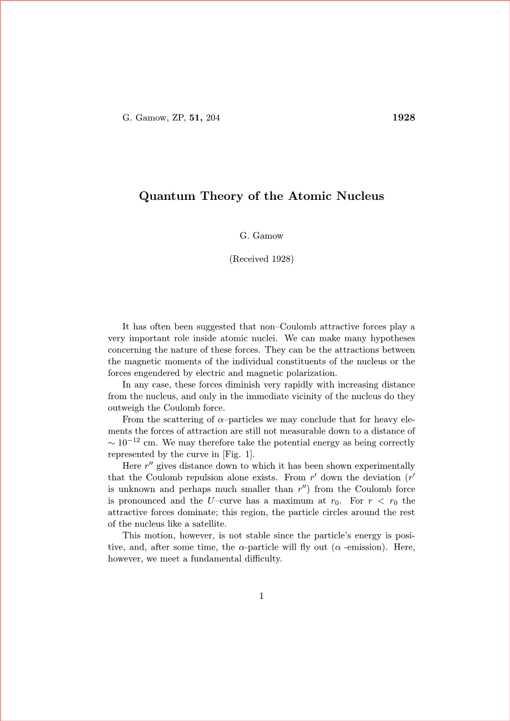
From the scattering of α–particles we may conclude that for heavy elements the forces of attraction are still not measurable down to a distance of ∼ 10−12 cm. We may therefore take the potential energy as being correctly represented by the curve in [Fig. 1].
Here r00 gives distance down to which it has been shown experimentally that the Coulomb repulsion alone exists. From r0 down the deviation (r0 is unknown and perhaps much smaller than r00) from the Coulomb force is pronounced and the U–curve has a maximum at r0. For r r0 the attractive forces dominate; this region, the particle circles around the rest of the nucleus like a satellite.
This motion, however, is not stable since the particle’s energy is positive, and, after some time, the α-particle will fly out (α -emission). Here, however, we meet a fundamental difficulty.
1Figure 1:
To fly off, the α–particle must overcome a potential barrier of height U0
[Fig. 1]; its energy may not be less than u0. But the energy of the emitted
α–particle, as verified experimentally, is much less. For example, we find on analyzing the scattering of Ra − c0 – α–particles by uranium that for the uranium nucleus the Coulomb law is valid down to distances of 3.2 × 10⁻¹² cm. on the other hand, the α-particles emitted by uranium itself have an energy which represents a distance of 3.2×10⁻¹² cm ( r2 in [Fig. 1] ) on the repulsive curve. If an α-particle, coming from the interior of the nucleus, is to fly away, it must pass through the region r1 and r2 where its kinetic energy would be negative, which, naturally, is impossible classically.
To overcome this difficulty, Rutherford assumed that the α-particles in the nucleus are neutral, since they are assumed to have two electrons there.
Only at a certain distance from the nucleus, on the other side of the potential barrier’s maximum, do they, according to Rutherford. lose their two electrons. which fall back into the nucleus while the α-particles fly on impelled by the Coulomb repulsion. But this assumption seems very unnatural, and can hardly be a true picture.
If we consider the problem from the wave mechanical point of view, the above difficulties disappear by themselves. In wave mechanics a particle always has a finite probability, different from zero, of going from one region to another region of the same energy, even through the two regions are separated by an arbitrarily large but finite potential barrier.
As we shall see further, the probability for such a transition, all things considered, is very small and, in fact, is smaller the higher the potential barrier is. To clarify this point, we shall analyze a simple case [see Fig. 2].
We have a rectangular potential barrier and we wish to find the solution
2Figure 2: of Schroedinger’s equation which represents the penetration of the particle from right to left. For the energy E we write the wave function ψ in the following form:
ψ = Ψ(q)e(2πi/h)Et
,where Ψ(q) satisfies the amplitude equation
∂2Ψ 8π2m
(E − U) Ψ = 0
+(1)
For the region I we have the solution
Ψ1 = A cos ·(kq + α)
∂q2 h2 where A and α are two arbitrary constants and √
√
2π 2m k =
·
E(2a) h
In the region II the solution reads
00
ΨII = B1e−k q + B2ek q where
√p
2π 2m k0 =
·
At the boundary q = 0 the following conditions apply:
U0 − E
(2b) h
ꢀꢁꢀꢁ
∂ΨI ∂ΨII
ΨI(0) = ΨII(0) and =,
∂q ∂q q=0 q=0
3from which we easily obtain
AA
B1 =
· sin(α + θ); B2 = −
· sin(α − θ),
2 sin θ 2 sin θ where
1qsin θ =
1 + (kk0 )2
The solution in region II therefore reads
A
00
ΨII
=
· [sin(α + θ) · ek q − sin(α − θ)ek q].
2 sin θ
In III we again have
ΨIII = C cos(kq + β)
At the boundary q = l we have from the boundary conditions
A
00
· [sin(α + θ)e−lk ] − sin(α − θ)e+lk ] = C cos(kl + β)
2 sin θ and
A
00k0 · [sin(α + θ)e−lk ] − sin(α − θ)e+lk ] = −kC sin(kl + β).
2 sin θ
Hence
(" #
ꢂꢃ
2
A2
4 sin2 θ k0 k
2lk0
C2 =
·
1 +
· sin2(α − θ) · e
"#
ꢂꢃ
2k0 k
− 1 − · 2 sin(α − θ) · sin(α + θ)
"#)
ꢂꢃ
2k0
0
· sin2(α + θ) · e−2lk
+ 1 + .(3) k
The calculation of β is of no interest to us. We are interested only in the case in which lk0 is very large so that we need consider only the firs term in
(3).
We thus have the following solution: left: right:
"#
1/2
ꢂꢃ
2sin(α − θ)
2 sin θ k0 k
0
A cos(kq + α) . . . A · 1 + · e+lk cos(kq + β).
4π
2
If we now write α − instead of α multiply the obtained solution by i, and then add the two solutions, we obtain on the left
Ψ = Aei(kq+α)
,(4a) on the right, however,
"#
Ψ =
· 1 +
1/2 · e+lk0 {sin(α − θ) cos(kq + β)−
ꢂꢃ
2
Ak0 k
2 sin θ
ꢄi cos(α + θ) cos(kq + β0) ,
(4b) where β0 is the new phase.
Eh
If we multiply this solution by e2πi t, we obtain for Ψ on the left the (from right to left) advancing wave; on the right, however, the complex
0oscillatory phenomenon with a very large amplitude (elk ) that departs only slightly from a standing wave. This means nothing other than that the wave coming from the right is partly reflected and partly transmitted.
We thus see that the amplitude of the transmitted wave is smaller the smaller is the total energy E, and in fact the factor
√
2π · 2m√
−lk0 U0−E .l he
= e plays an important role in this connection.
We can now solve the problem for two symmetrical potential barriers
[Fig. 3]. We shall seek two solution.
Figure 3:
One solution is to be valid for positive q, and for q q0 + l is to give the wave:
i( 2πE t−kq+α) h
Ae
5The other solution is valid for negative q, and for q −(q0 + l) gives the wave
ꢅꢆ
2πEl+qk0−α
Aei
.h
We cannot attach the two solutions each other continuously at q = 0 since we have here two boundary conditions to fulfill and only one arbitrary constant
α to adjust. The physical reason for this impossibility is that the Ψ – function constructed from these two solutions does not satisfy the conservation law
+(q0+l)
Z
ꢇꢈ
∂
−h
¯¯¯
ψψdq = 2 ·
ψ grad ψ − ψ grad ψ
I
∂t
4π · i · m
−(q0+l)
To overcome these difficulties we must assume that the vibrations are damped and make E complex hλ
E = E0 + i
4π where E0 is the usual energy and λ is the damping decrement (decay constant). We then see from the relations (2a) and (2b) that k and k0 are complex, that is, that the amplitude of our wave also depends exponentially on the coordinate q. For example, for the running wave the amplitude in the direction of the diverging wave will increase. This means nothing more than that if the vibrations are damped at the source of the wave, the amplitude of the wave segment that left earlier must be larger.
We can now determine α so that the boundary conditions are fulfilled.
Eh
But the exact solution does not interest us. If λ is small compared to
h
E10−5
(forRa − c0 sec−1 = 1022sec−1 and λ = 105sec−1) the change
∼
=
10−27
− α
2 t in Ψ(q) is very small and we can simply multiply the old solution with e
The conservation principle then reads
.
+(q0+l)
Z
∂
A2h
(q) (q)
II,III II, III e−λt
· Ψ dq = −2
· 2ik · e−λt
Ψ,
∂t
4π · i · m
−(q0+l) from which we obtain
√h
− 4πl 2m√
4hk sin2 θ
U0−E
ꢀꢁ
λ =
· e
,(5)
where k is a number of order of magnitude one.
ꢅꢆ
2k0 k0
πm 1 + 2(l + q0)k
6This formula gives the dependence of the decay constant on the decay energy for our simple nuclear model.
Now we can go over to the case of the actual nucleus.
We cannot solve the corresponding wave equation because we do not know the exact formula for the potential in the neighborhood of the nucleus.
But even without an exact knowledge of the potential we can carry over to the actual nucleus results obtained from our simple model.
As usual, in the case of a central force, we seek the solution in polar coordinates and, in fact, in the form
Ψ = u(θ, φ)χ(r).
For u we obtain the spherical harmonics, and χ must satisfy the differential equation
"#d2χ 2 dχ 8π2m h2
8π2m n(n + 1)
+
+
· E − U −
·
· χ = 0, dr2 r dr h2 r2 where n is the order of the spherical harmonic. We can place n = 0, since if n 0, this would really be just as through the potential energy were enlarged, and because of this damping for these oscillations is much smaller.
The particle must first pass over to the state n = 0 and can only then fly away.
It is quite possible that such transitions are the cause of the γ rays which always accompany α – emission. The probable shape of U is shown in [Fig.
4].
For large values of r, we shall take for χ the solution
i( eπE t−kr)
Ah
χI = · e r
Even through we cannot obtain the exact solution of the problem in this case, we can still say that on the average in the regions I and I0, χ does not decrease very rapidly (in the three dimensional case like l/r).
In the region III, however, χ decreases exponentially, and in analogy with our simple case we may state that the relation between the amplitude decrease and E is given by the factor
√hr2
Z
− 2π 2m
√e
U − E dr r1
7Figure 4:
If we use the conservation principle we can again write down the formula
√hr2
Z
− 2π 2m
√
λ = D . e
U − Edr
(6) r1 where D depends on the particular properties of the nuclear model. We can neglect the dependence of D on E compared to its exponential dependence.
We may also replace the integral r2
Z
√
U − E dr r1 by the approximate integral
2Ze2 s
E
Z
2Ze2
− E · dr r
0qr1 r2
The relative error we introduce in this way is of the order of . Since r1/r2 is small, this error is not very large. Since E does not differ much for different radioactive elements, we write as an approximation log λ = constE + BE . ∆E,
8. . . where
√hE3/2
π2 2m · 2Ze2
BE =
.(7)
We wish to compare this formula with the experimental results. It is known that if we plot the logarithm of the decay constant against the energy of the emitted α-particle, all the points for a definite radioactive family fall on a straight line. For different families we obtain different parallel lines.
The empirical formula reads log λ = const + bE where b is a constant that is common to all radioactive families.
The experimental value of b is bexp = 1.02 × 10⁷ (calculated from Ra–A and Ra).
If we put the energy value for Ra–A into our formula, we get btheoretical = 0.7 × 10⁷
This order of magnitude agreement shows that the basic assumptions of our theory must be correct . . .
9
Quantum Theory of the Atomic Nucleus