Introductory Review of Cosmic Inflation

Introductory Review of Cosmic Inﬂation
Shinji Tsujikawa1
Research Center for the Early Universe, University of Tokyo,
Hongo, Bunkyo-ku, Tokyo 113-0033, Japan
Abstract
These lecture notes provide an introduction to cosmic inﬂation. In particular I will review the basic concepts of inﬂation, generation of density perturbations, and reheating after inﬂation.
1email: shinji@resceu.s.u-tokyo.ac.jp, shinji@gravity.phys.waseda.ac.jp 1 Preface
These lecture notes are based on invited lectures at The Second Tah Poe School on Cosmology
“Modern Cosmology”, Naresuan University, Phitsanulok, Thailand, April 17 -25, 2003. See the web page
for the details of this school and conference.
2 Introduction
The proposal of General Relativity by Einstein in 1915 made it possible to discuss the structure of spacetime and the evolution of the universe in terms of physical laws. In 1922 Friedmann found the existence of expanding/collapsing cosmological solutions by solving the Einstein ﬁeld equations. In 1929 Hubble discovered the expansion of the universe by the observations in the redshift of galaxies, as the Einstein theory predicts. In 1946 Gamov and his collaborators showed that the universe must begin in a very hot and dense state from the theory of nucleosynthesis.
They also predicted that the present universe should be ﬁlled with the microwaves with black body radiations. In 1965 Penzias and Wilson discovered microwave background radiations which coincide well with theoretical predictions by Gamov et al.. These strong observational evidences have made people believe that the universe started out from a hot and dense state, which is called as the standard big-bang model.
In standard big-bang cosmology the state of the universe is characterized by the radiationdominated or the matter-dominated stage. These correspond to the decelerated expansion of the universe where the second derivative of the scale factor is negative. Meanwhile this decelerated expansion is not suﬃcient to solve a number of cosmological problems such as ﬂatness and horizon problems which plagues in the standard big-bang scenario2. In order to overcome these fundamental problems, it is required to consider an epoch of accelerated expansion in the early universe, i.e., inﬂation.
The basic ideas of inﬂation were originally proposed by Guth [1] and Sato [2] independently in 1981, which is now termed as old inﬂation3. This corresponds to the de-Sitter inﬂation which makes use of the ﬁrst-order transition to true vacuum. However, it has a serious shortcoming that the universe becomes inhomogeneous by the bubble collision soon after the inﬂation ends.
The revised version was proposed by Linde [4], and Albrecht and Steinhardt [5] in 1982, which is dubbed as new inﬂation. This corresponds to the slow-roll inﬂation with the second-order transition to true vacuum. Unfortunately this scenario also suﬀers from a ﬁne-tuning problem of spending enough time in false vacuum to lead to suﬃcient amount of inﬂation. In 1983 Linde [6] considered the variant version of the slow-roll inﬂation called chaotic inﬂation, in which initial conditions of scalar ﬁelds are chaotic. According to this model, our homogeneous and isotropic universe may be produced in the regions where inﬂation occurs suﬃciently. While old and new inﬂation models are based on the assumption that the universe was in a state of thermal equilibrium from the beginning, chaotic inﬂation can occur even without such an assumption.
In addition chaotic inﬂation can start out in the regime close to Planck density, thereby solving the problem of initial conditions.
2In the next section I will explain how inﬂation solves these problems.
3Note that a speciﬁc version of the inﬂationary scenario–so called R2 inﬂation– was proposed by Starobinsky one year earlier [3]. Nevertheless this did not explicitly point out the virtue of inﬂation as in the paper of Guth.
2Many kinds of inﬂationary models have been constructed in these twenty years (see e.g., ref. [7, 8]). In particular, the recent trend is to construct consistent models of inﬂation based on superstring or supergravity models. See ref. [9] for a review in such a direction.
The inﬂationary paradigm not only provides an excellent way in solving ﬂatness and horizon problems but also generates density perturbations as seeds for large scale structure in the universe [10]. In fact inﬂation provides a causal mechanism to generate nearly scale-invariant spectra of cosmological perturbations. Quantum ﬂuctuations of the ﬁeld driving inﬂation–called inﬂaton– are typically frozen by the accelerating expansion when the scales of ﬂuctuations leave the Hubble radius. Long after the inﬂation ends, the scales cross inside the Hubble radius again. Thus perturbations imprinted during inﬂation can be the origin of large-scale structure in the universe. In fact temperature anisotropies observed by the COBE satellite in 1992 exhibit nearly scale-invariant spectra as predicted by the inﬂationary paradigm. Recent observations of WMAP also show strong evidence for inﬂation [11].
3 The standard big-bang cosmology and its problems
3.1 The standard big-bang cosmology
The standard big-bang cosmology is based on the cosmological principle [8], which means that the universe is homogeneous and isotropic on large distance. Then the metric takes the Friedmann-
Robertson-Walker (FRW) form:
"#dr2
1 − Kr2 ds2 = gµνdxµdxν = −dt2 + a2(t) (1)
+ r2(dθ2 + sin2 θdφ2) .
Here a(t) is the scale factor with t being the cosmic time. The constant K is the spatial curvature, where positive, zero, and negative values correspond to closed, ﬂat, and open universes, respectively.
The evolution of the universe is dependent on the material within it. This is characterized by the equation of state between the energy density ρ(t) and the pressure p(t). Typical examples are : p = ρ/3 , radiation , (2) p = 0 , dust . (3)
In order to know the dynamical evolution of the universe, it is required to solve the Einstein equations in General Relativity. The Einstein equations are expressed as [12, 13]
1
2
Gµν ≡ Rµν − gµνR = 8πGTµν − Λgµν,
(4) where Rµν, R, Tµν, and G are the Ricci tensor, Ricci scalar, energy momentum tensor, gravitational constant, respectively. The Planck energy, mpl = 1.2211 × 1019 GeV, is related with G through the relation mpl = (¯hc5/G)1/2. Here ¯h and c are the Planck’s constant and the speed of light, respectively. Hereafter we use the units ¯h = c = 1. Λ is a cosmological constant originally introduced by Einstein.
3For the background metric (1) with a negligible cosmological constant, the Einstein equations
(4) yield
8π
3m2pl
Ka2
H2 = (5)
ρ −
,
ρ˙ + 3H(ρ + p) = 0 , (6)
where a dot denotes the derivative with respect to t, and H ≡ a˙/a is the Hubble expansion rate.
Eqs. (5) and (6) are so called the Friedmann and Fluid equations, respectively. Combining these relations gives the following equation, a¨ a
4π
3m2pl
= − (ρ + 3p) . (7)
The Friedmann equation (5) can be rewritten as
Ka2H2
Ω − 1 = (8)
,
where
3H2m2pl
8π
ρ
Ω ≡ (9) with
ρc ≡
,.
ρc
Here the density parameter Ω is the ratio of the energy density to the critical density. When the spatial geometry is ﬂat (K = 0), the solutions for Eqs. (5) and (6) are
a ∝ t1/2 a ∝ t2/3
ρ ∝ a−4
ρ ∝ a−3
,,
Radiation dominant : (10)
Dust dominant : (11)
,.
In these simple cases, the universe is expanding deceleratedly (¨a 0) as conﬁrmed by Eq. (7).
3.2 Problems of the standard big-bang cosmology
3.2.1 Flatness problem
In the standard big-bang theory with a¨ 0, the a2H2(= a˙2) term in Eq. (8) always decreases.
This indicates that Ω tends to shift away from unity with the expansion of the universe. However, since present observations suggest that Ω is within the order of magnitude of one [11], Ω needs to be very close to one in the past. For example, we require |Ω − 1| O(10−16) at the epoch of nucleosynthesis [8, 14] and |Ω−1| O(10−64) at the Planck epoch [15]. This is an extreme ﬁnetuning of initial conditions. Unless initial conditions are chosen very accurately, the universe soon collapses, or expands quickly before the structure can be formed. This is so called the ﬂatness problem.
43.2.2 Horizon problem
Consider a comoving wavelength, λ, and also a physical wavelength, aλ, which is inside the Hubble radius, H−1 (i.e., aλ
H
−1). The standard big-bang cosmology is characterized by the ∼cosmic evolution of a ∝ tp with 0 p 1. In this case the physical wavelength grows as aλ ∝ tp, whereas the Hubble radius evolves as H−1 ∝ t. Therefore the physical wavelength becomes much smaller than the Hubble radius with the passage of time. This means that the region where the causality works eventually becomes the only small fraction of the Hubble radius.
To be more precise, let us ﬁrst deﬁne the particle horizon DH(t) where the light travels from the beginning of the universe, t = t∗,
Ztdt
DH (t) = a(t)dH (t) , (12) with dH (t) =
.
a(t) t
∗
Here dH(t) corresponds to the comoving distance. Setting t∗ = 0, we ﬁnd dH(t) = 3t in the matter-dominant era. We observe photons in the Cosmic Microwave Background (CMB) which are emitted at the time of decoupling. The particle horizon at decoupling, DH (tdec) = a(tdec)dH (tdec), corresponds to the region where photons could have contacted causally at that time. The ratio of dH (tdec) to the particle horizon today, dH(t0), where t0 is the present time, is estimated as
!
1/3
ꢀꢁ
1/3 dH(tdec )105 dH(t0) 1010
t0
≈≈
≈ 10−2 (13)
.
tdec
This result implies that the causality regions of photons are restricted to be small. In fact the surface of the last scattering surface only corresponds to the angle of order 1◦. Observationally, however, we see photons which thermalize to the same temperature in all regions in the CMB sky. This is so called the horizon problem.
3.2.3 The origin of large-scale structure in the universe
The COBE satellite observes the anisotropies in the last scattering surface, whose amplitudes are small and close to scale-invariant. These ﬂuctuations spread so large a scale that it is practically impossible to generate them between the big bang and the time of the last scattering in the standard cosmology. This problem is almost equivalent to the horizon problem mentioned above, i.e., the standard cosmology can not provide satisfactory explanation for the origin of large-scale structure.
3.2.4 Monopole problem
According to the view point of particle physics, the breaking of supersymmetry leads to the production of many unwanted relics such as monopoles, cosmic strings, and topological defects
[7]. The string theories also predict supersymmetric particles such as gravitinos, Kaluza-Klein particles, and moduli ﬁelds.
If these particles exist in the early stage of the universe, the energy densities of them decrease as a matter component (∼ a−3). Since the radiation energy density decreases as ∼ a−4 in the radiation-dominant era, these massive relics could be the dominant materials in the universe, which contradicts with observations. This problem is generally called as the monopole problem.
54 Idea of inﬂationary cosmology
The problems in the big-bang cosmology lie in the fact that the universe always exhibits the decelerating expansion. Let us assume the existence of a stage in the early universe with an accelerated expansion of the universe, i.e., a¨ 0 . (14)
From the relation (7) this corresponds to the condition
ρ + 3p 0 . (15)
The condition (14) essentially means that a˙ (= aH) increases during inﬂation. Then the comoving Hubble radius, (aH)−1, decreases in the inﬂationary phase. This property is the key point to solve the cosmological puzzles in the standard big-bang cosmology as I will show below.
4.1 Flatness problem
Since the a2H2 term in Eq. (8) increases during inﬂation, Ω rapidly approaches unity. After the inﬂationary period ends, the evolution of the universe is followed by the conventional big-bang phase and |Ω−1| begins to increase. In spite of this, as long as the inﬂationary expansion occurs suﬃciently and makes Ω very close to one, Ω stays of order unity even in the present epoch.
4.2 Horizon problem
Since the scale factor evolves as a ∝ tp with p 1 during inﬂation, the physical wavelength, aλ, grows faster than the Hubble radius, H−1(∝ t). Therefore the physical wavelength is pushed outside the Hubble radius during inﬂation. This means that the region where the causality works is stretched on scales much larger than the Hubble radius, thus solving the horizon problem.
Of course the Hubble radius begins to grow faster than the physical wavelength after inﬂation
(radiation/matter dominant era). In order to solve the horizon problem, it is required that the following condition is satisﬁed for the comoving particle horizon:
ZZtdec t0 dt dt
ꢀ
.
(16) a(t) a(t) ttdec
∗
This implies that the comoving distance that photons can travel before decoupling needs to be much larger than that after the decoupling. According to the precise calculation, it is achieved when the universe expands about e70 times during inﬂation [8, 15].
4.3 The origin of the large scale structure
The fact that the comoving Hubble radius decreases during inﬂation makes it possible to generate the nearly scale-invariant density perturbations on large scales. Since the scales of perturbations are within the Hubble radius in the early stage of inﬂation, causal physics works to generate small quantum ﬂuctuations. After a scale is pushed outside the Hubble radius (i.e., the ﬁrst horizon crossing) during inﬂation, the perturbations can be described by classical ones. When the inﬂationary period ends, the evolution of the universe is followed by the standard big-bang cosmology, and the comoving Hubble radius begins to increase. Then the scales of perturbations
6cross inside the Hubble radius again (the second horizon crossing), after which causality works.
The small perturbations imprinted during inﬂation appear as large-scale perturbations after the second horizon crossing. In this way the inﬂationary paradigm naturally provides a causal mechanism in generating the seeds of density perturbations observed in the CMB anisotropies.
4.4 Monopole problem
During the inﬂationary phase (ρ + 3p 0), the energy density of the universe decreases very slowly. For example, when the universe evolves as a ∝ tp with p 1, we have H ∝ t−1 ∝ a−1/p and ρ ∝ a−2/p. Meanwhile the energy density of massive particles decreases much faster (∼ a−3), these particles are red-shifted away during inﬂation, thereby solving the monopole problem.
Of course, we have to worry for the case where these unwanted particles are produced after inﬂation. In the process of reheating followed by inﬂation, the energy of the universe can be transferred to radiation or other light particles. At this stage unwanted particles must not be overproduced in order not to violate the success of the standard cosmology such as nucleosynthesis. Generally if the reheating temperature is suﬃciently low, the thermal production of unwanted relics such as gravitinos can be avoided.
5 Inﬂationary dynamics
The scalar ﬁelds are the important ingredients in particle physics theories. Consider a homogeneous scalar ﬁeld, φ, called inﬂaton, whose potential energy leads to the exponential expansion of the universe. The energy density and the pressure density of the inﬂaton can be described, respectively, as
11
22
22
˙˙
ρ = φ + V (φ) , p = φ − V (φ) , (17)
where V (φ) is the potential of the inﬂaton. Substituting Eq. (17) for Eqs. (5) and (6), we get
ꢂꢃ
8π 1
2
H2 = (18)
φ + V (φ) ,
˙
3m2pl 2
0
¨˙
φ + 3Hφ + V (φ) = 0 , (19) where κ2 ≡ 8πG = 8π/mp2l, and we neglected the curvature term K2/a2 in Eq. (18).
2
˙
During inﬂation, the relation (15) yields φ V (φ), which indicates that the potential energy of the inﬂaton dominates over the kinetic energy of it. Therefore a ﬂat potential of the inﬂaton is required in order to lead to suﬃcient amount of inﬂation. Imposing the slow-roll conditions:
1
2
˙¨˙
2φ ꢁ V (φ) and φ ꢁ 3Hφ, Eqs. (18) and (19) are approximately given as
8π
H2 '
V (φ), (20)
3m2pl
0
˙
3Hφ ' −V (φ). (21)
7Deﬁning the so-called slow-roll parameters
ꢀꢁ2 m2pl m2 00
V 0 V
Vpl
ꢀ ≡
η ≡
,,
(22)
16π 8π V we can easily verify that the above slow-roll approximations are valid when
ꢀ ꢁ 1, |η| ꢁ 1 . (23)
The inﬂationary phase ends when ꢀ and |η| grow of order unity. A useful quantity to describe the amount of inﬂation is the number of e-foldings, deﬁned by
Ztf af
N ≡ ln
Hdt ,
=(24) ai ti where the subscripts i and f denote the quantities at the beginning and the end of the inﬂation, respectively.
−60
In order to solve the ﬂatness problem, Ω is required to be |Ωf − 1| 10 right after the ∼end of inﬂation. Meanwhile the ratio |Ω − 1| between the initial and ﬁnal phase of inﬂation is given by
!
2
|Ωf − 1|
|Ωi − 1| ai
'
= e−2N (25)
,
af where we used the fact that H is nearly constant during inﬂation. Assuming that |Ωi − 1| is of order unity, the number of e-foldings is required to be N 70 to solve the ﬂatness problem. We
∼have similar number of e-foldings from the requirement to solve the horizon problem.
6 Models of inﬂation
So far we did not mention the form of the inﬂaton potential, V (φ). Originating from the old inﬂationary scenario proposed by Guth [1] and Sato [2], we now have varieties of inﬂationary models : R2, new, chaotic, extended, power-law, hybrid, natural, supernatural, extranatural, eternal, D-term, F-term, brane, oscillating, trace-anomaly driven,..., etc.
These diﬀerent kinds of models can be roughly classiﬁed in the following way [16]. The ﬁrst class (type I) is the “large ﬁeld” model, in which the initial value of the inﬂaton is large and it rolls down toward the potential minimum at smaller φ. Chaotic inﬂation [6] is one of the representative models of this class. The second class (type II) is the “small ﬁeld” model, in which the inﬂaton ﬁeld is small initially and slowly evolves toward the potential minimum at larger φ. New inﬂation [4, 5] and natural inﬂation [17] are the examples of this type. In the ﬁrst model, the second derivative of the potential V (2)(φ) usually takes positive values, whereas
V (2)(φ) can change its sign in the second model. The third one (type III) is the hybrid (double) inﬂation model [18], in which inﬂation typically ends by the phase transition triggered by the presence of the second scalar ﬁeld (or by the second phase of inﬂation after the phase transition).
Let us brieﬂy recap each type of inﬂationary models.
86.0.1 Chaotic inﬂation– an example of type I
The chaotic inﬂation model is described by the quadratic or quartic inﬂaton potential,
11
24
V (φ) = m2φ2 , or V (φ) = λφ4 . (26)
The “chaotic” means that initial conditions of inﬂaton are distributed chaotically. According to this scenario, the region which undergoes the suﬃcient amount of inﬂation gives rise to our universe.
Let us investigate the evolution of the universe in the case of the quadratic potential. Then
Eqs. (20) and (21) read
4πm2φ2
3m2pl
2
H2 '
,
3Hφ + m φ ' 0 . (27)
˙
Combining these relations gives the following solutions: mmpl
√
φ ' φi − t ,
(28)
2 3π
"#r
ꢀꢁ
π m mmpl t2 ,
√a ' ai exp 2 (29)
φit −
3 mpl
4 3π where φi is an integration constant corresponding to the initial values of the inﬂaton. We
ﬁnd from the relation (29) that the universe expands exponentially during the initial stage of inﬂation. With the increase of the second term in the square bracket of Eq. (29), the expansion rate slows down. Since the slow-roll parameters are expressed as m2pl
4πφ2
ꢀ = η =
,
(30)
√the inﬂationary period ends around |φ| ≈ mpl/ 4π, after which the system enters a reheating stage. The total amount of inﬂation is approximately expressed as
!
2
φi
1
− .
2
N ' 2π (31) mpl
In order to lead to suﬃcient inﬂation N 3mpl.
70, we require the initial value to be φi
∼
∼
The inﬂaton mass, m, is constrained by the amplitude of density perturbations observed by the COBE satellite. In order to ﬁt observations, m is required to be [8] m ' 10−6mpl . (32)
In the quartic potential case, the self-coupling is constrained to be λ ' 10−13 by the similar argument [7, 8].
9V(
)
φ
0
φ
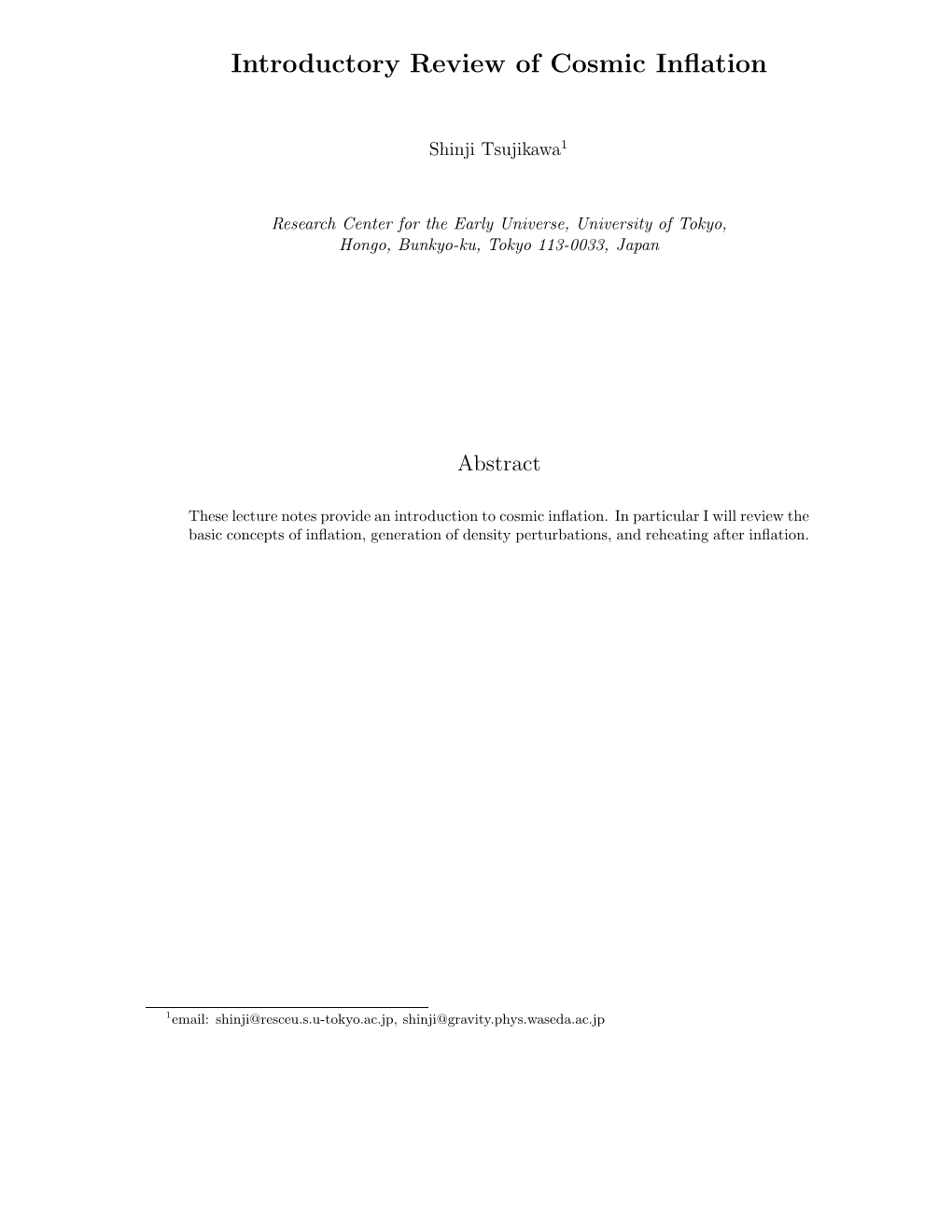
Figure 1: The schematic illustration of the potential of the chaotic inﬂation model. This belongs to the class of the “large ﬁeld” model.
6.0.2 Natural inﬂation– an example of type II
Natural inﬂation model [17] is characterized by Pseudo Nambu-Goldstone bosons (PNGBs) which appear when an approximate global symmetry is spontaneously broken. The PNGB potential is expressed as
ꢂꢀꢁꢃ
φf
V (φ) = m4 1 + cos
,
(33) where two mass scales m and f characterize the height and width of the potential, respectively.
The typical mass scales are of order f ∼ mpl ∼ 1019 GeV and m ∼ mGUT ∼ 1016 GeV, which are expected by particle physics.
Let us consider the case where the inﬂaton is initially located in the region, 0 φ πf, and inﬂation occurs while the inﬂaton slowly evolves toward the potential minimum at φ = πf.
The slow-roll parameters are
ꢂꢃ2 m2pl m2pl sin(φ/f) cos(φ/f)
ꢀ =
,.
η = − (34)
16πf2 1 + cos(φ/f)
8πf2 1 + cos(φ/f)
Note that ꢀ and η depend on f, but not on m. Inﬂation starts out from the regime where φ is close to zero. The system enters a reheating stage when the inﬂaton begins to oscillate around
φ = πf.
One typical property in the type II model is that the second derivative of the inﬂaton potential can change its sign. In the natural inﬂation, V (2)(φ) is negative when inﬂaton evolves in the region of 0 φ πf/2. This leads to the enhancement of inﬂaton ﬂuctuations by spinodal (tachyonic) instability [19, 20, 21]. When the particle creation by spinodal instability is neglected, the number of e-foldings is expressed by [17]
ꢂꢃ
16πf2 m2pl sin(φf /2f) sin(φi/2f)
,
N = ln (35)
10 V(φ)
0
πf
φ
Figure 2: The schematic illustration of the potential of the natural inﬂation model. This belongs to the class of the “small ﬁeld” model. where φi and φf are the initial and ﬁnal values of the inﬂaton during inﬂation, respectively. In
order to obtain the suﬃcient amount of e-foldings satisfying N
70, the initial value of the ∼
inﬂaton is required to be φ(ti) 0.1mpl for the mass scale f ∼ mpl.
∼
6.0.3 Hybrid (Double) inﬂation– an example of type III
The inﬂationary model building in the presence of multiple scalar ﬁelds is the recent trend from the viewpoint of particle physics [9]. Let us consider the Linde’s hybrid inﬂation model [18], described by
!
2
λ
M2
λ
11
V =
χ2 −
+ g2φ2χ2 + m2φ2 . (36)
422
When φ2 is large, the ﬁeld tends to roll down toward the potential minimum at χ = 0. In this case, the potential is eﬀectively described by a single ﬁeld,
M4
1
V '
+ m2φ2 . (37)
4λ 2
Inﬂation does not end for the potential (37). In the presence of the χ ﬁeld, however, the mass of the ﬁeld χ becomes negative for φ φc ≡ M/g. Then the ﬁeld begins to roll down to
√one of the true minima at φ = 0 and χ = ±M/ λ (see Fig. 3). The original version of the hybrid inﬂation [18] corresponds to the case where the inﬂation soon comes to an end after the symmetry breaking (φ φc) due to the rapid rolling of the ﬁeld χ. In this case the number of e-foldings acquired in double inﬂation can be approximately estimated by using the potential
(37):
2πM4
φi
N ' ,ln (38)
λm2m2pl φc
11 V
φ
φc
χ
0
Figure 3: The schematic illustration of the potential of the hybrid (double) inﬂation model.
This model is characterized by multiple scalar ﬁelds. where φi is the initial value of inﬂaton.
If the condition, M2 ꢀ λMp2, is satisﬁed, the mass of the ﬁeld χ is “light” relative to the Hubble rate around φ = φc, thereby leading to the second stage of inﬂation for φ φc [22]. This corresponds to the double inﬂationary scenario.
7 Density perturbations from inﬂation
In this section we study cosmological perturbations generated from inﬂation. For simplicity we shall consider the single-ﬁeld model of inﬂation. The most general form of the line element that describes scalar metric perturbations is written as [23, 24] ds2 = a2(τ){−(1 + 2A)dτ2 + 2B,i dxidτ + [(1 − 2ψ)γij + 2E,ij ]dxidxj} , (39)