How to Generate a List of Sheet Names from a Workbook Without VBA

How To Generate A List Of Sheet Names From A Workbook Without VBA

This can be pretty handy if you have a large workbook with hundreds of sheets and you want to create a table of contents. This method uses the little known and often forgotten Excel 4 macro functions.

These functions aren’t like Excel’s other functions such as SUM, VLOOKUP, INDEX etc. These functions won’t work in a regular sheet, they only work in named functions and macro sheets. For this trick we’re going to use one of these in a named function.

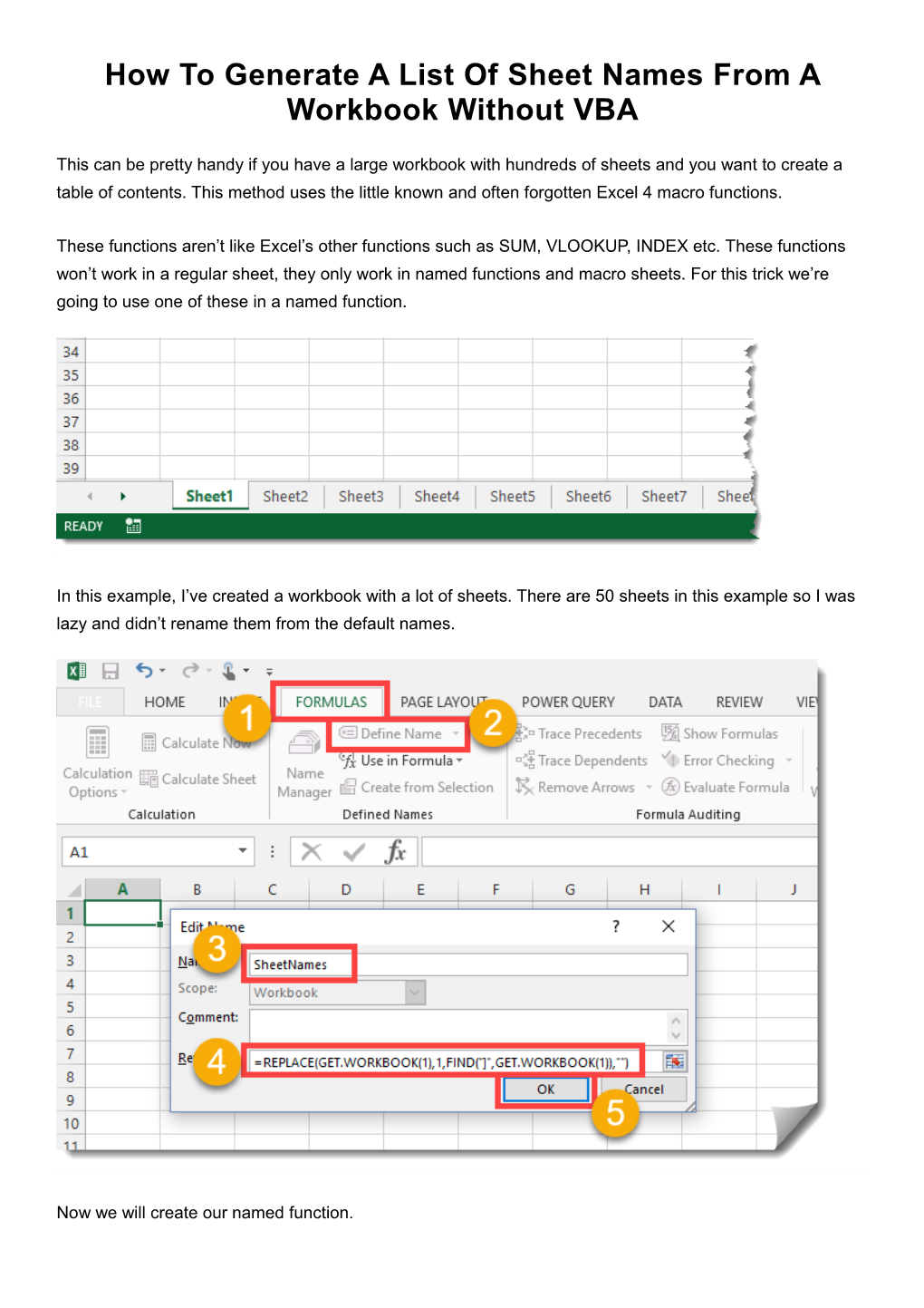
In this example, I’ve created a workbook with a lot of sheets. There are 50 sheets in this example so I was lazy and didn’t rename them from the default names.

Now we will create our named function.

1. Go to the Formulas tab.
2. Press the Define Name button.
3. Enter SheetNames into the name field.
4. Enter the following formula into the Refers to field.

=REPLACE(GET.WORKBOOK(1),1,FIND("]",GET.WORKBOOK(1)),"")

1. Hit the OK button.

In a sheet within the workbook enter the numbers 1,2,3,etc… into column A starting at row 2 and then in cell B2 enter the following formula and copy and paste it down the column until you have a list of all your sheet names.

=INDEX(SheetNames,A2)

As a bonus, we can also create a hyperlink so that if you click on the link it will take you to that sheet. This can be handy for navigating through a spreadsheet with lots of sheets. To do this add this formula into the column C.

=HYPERLINK("#'"&B2&"'!A1","Go To Sheet")

Note, to use this method you will need to save the file as a macro enabled workbook (.xls, .xlsm or .xlsb). Not too difficult and no VBA needed.