Gauge Theory on a Lattice

Gauge Theory on a Lattice
One approach to ﬁeld theory, in particular to aspects that are not well treated in perturbation theory, is to approximate the ﬁeld deﬁned on a spacetime continuum with a lattice ﬁeld theory, deﬁned on a lattice of space-time points. There has been a great deal of cross-fertilization from considering renormalization from the continuum high-energy physics point of view and from the condensed matter, Wilsonian, viewpoint, in which the ﬁeld theory only makes sense down to some small distance scale anyway. But we are going to consider it for a diﬀerent reason — because it helps to clarify the fundamental idea of gauge ﬁelds.
Symmetry
Consider a theory which involves a set of N ﬁelds φi(xµ) which have an internal symmetry group G under which they transform with a representation
M, so that
X
G : φi(x) → φ′i(x) = (1)
Mij(G)φj(x).
j
If it is a symmetry, the Lagrangian must be invariant. For the kinetic
P
1
2term µ,i ∂µφi∂µφi, invariance requires that M is an orthogonal matrix
P
k MkiMkj = δij. That condition also insures the invariance of the mass
PPterm −12 i φ2i , and of any other “potential” term V ( i φi2) depending only on the “length” of φ. Provided V has that form, we see that the theory should be invariant under the orthogonal transformations (1). We see that the individual components φi are only projections along the unit vectors of an arbitrary orthonormal basis of RN , and do not have separate intrinsic physical meanings.
Discretization
How might we approximate the continuum theory on a lattice? Instead of φi(x) deﬁned for all values of x ∈ R4, we might have φi(~n) discrete variables deﬁned only for integer values ~n ∈ Z4, representing a lattice in space-time with lattice spacing a, with xµ = anµ. The mass term in the action
Z
XX X
11d4x −φ2i (x) → − a4
22
φ2i (~n).
~n∈Z4 ii
1For the kinetic energy term we need to replace a derivative by a ﬁnite diﬀerence. The simplest substitution is to replace
ꢀꢁ
1
~
∂µφi(x) →
φi(~n + ∆µ) − φi(~n) , awhere ∆µ is 1 in the µ direction and 0 in the others. Here the relation of xµ
1and ~n is xν = anν + aδµν, representing most accurately the x in the middle
2of the two lattice points. If we expand out the squares of the diﬀerences, we get terms which look just like the mass terms, but also nearest neighbor
Pcouplings i φi(~n + ∆µ)φi(~n).
Each of these contributions to the action is still invariant under the transformation (1), providing we use the same group transformation at every point in space-time. This is called a global gauge transformation.
In a relativistic ﬁeld theory, all information is local, because information can only travel at the speed of light. So we might ask, if the theory is unchanged by a group action at one point, why should that depend on having the same transformation at every other point? In other words, could we have a local symmetry, in which equation (1) holds with the group element varying from one point of space-time to another? The mass terms and other terms in V (φ) only depend on one point, so they don’t care whether M varies, and they are invariant under such transformations. But the nearest-neighbor coupling
X
φi(~n + ∆µ)φi(~n) → Mik(G(~n + ∆µ))Mij(G(~n)) φk(~n + ∆µ)φj(~n) iis not invariant because
M−1(G(~n + ∆µ))M(G(~n)) = 1 if the G’s (and hence the M’s) vary from point to point.
Parallel Transport
The problem is that we have a term in the Lagrangian that is a function of how φ changes from point to point, but we measure that change by how much the components change. That is only correct if the basis for comparing the φ’s does not change. We must have a way to measure change from point to point, but before we can subtract one φ vector from another at a diﬀerent
2point, we must “parallel transport” it to that new point. That is, for each link between neighboring points, we must have a rule for parallel transporting
φ ﬁelds from one end of the link to the other. This introduces new degrees of freedom, which are actually one element of the symmetry group (and
1
2therefore perhaps several degrees of freedom, N(N − 1) for SO(N), the orthogonal transformations in N dimensions). We can then build a theory with a local symmetry, but at the expense of introducing a lot of new degrees of freedom.
The theory that emerges from these consideration is a gauge ﬁeld theory. Its degrees of freedom include not only the “matter ﬁelds” at each site of the lattice, but also “gauge ﬁelds” on each link between nearest neighbors.
The matter ﬁelds live in a vector space which transforms linearly as a representation1 of the “gauge group” G. The gauge ﬁelds live in the group itself, at least in the lattice ﬁeld theory, but may alternately be considered to take values in the Lie algebra of generators of the group.
What is the meaning that the group element G associated with a given link
~
(~n, ~n+∆µ)? We called it a parallel transport, a deﬁnition of how one can transport e’
~the basis vectors ~ei(~n) to the point ~n + ∆µ rwhile keeping them parallel, and then reexpressing them in terms of the basis vectors
~ei(~n + ∆µ). Perhaps this is confusing, and you might ask why the basis vectors ~ei(~n) are not each identical to the corresponding
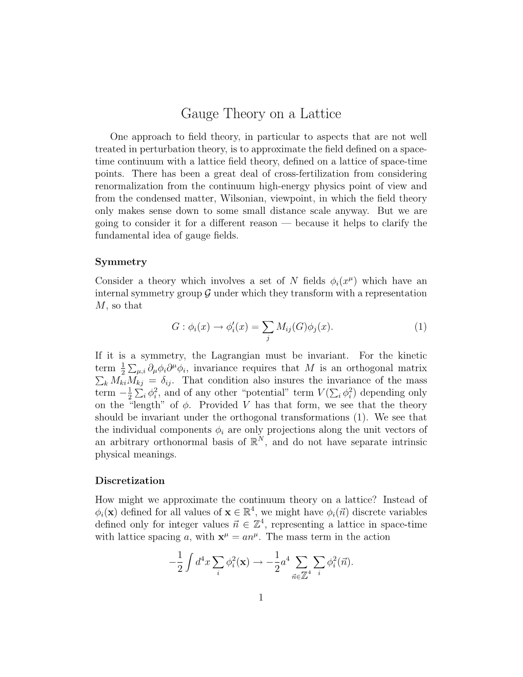
~ei(~n + ∆µ). It might help to think of an ordinary vector in the plane, expressed in polar coordinates. Consider the unit basis vector ~er at the point P. If we transport it to the point P′ while keeping it parallel to what it was, we arrive at the vector labelled Ger, which is not the same as the unit radial vector e′r at the point P′.
G e r
P’
Ge
θer
P
1To a physicist, the vector space in which the matter ﬁelds live is called the representation, but to mathematicians the representation consists of the matrices Mij, or more accurately the mapping from elements of the group into matrices, G → M(G).
3Covariant Derivative
When a group element G acts on a vector V =
P
~
Vieˆ which transforms iiunder a representation M, the components of the new vector are multiplied by the matrix:
X
X
Mij(G)Vjeˆ , so Vi′ =
Mij(G)Vj.
′
~~
G : V → V = iij j
~
~
So if G parallel transports φ(~n) from ~n to ~n + ∆µ, and if we subtract this
~from φ(~n + ∆µ) to get the change in φ, we have

XX

∆φ = φi(~n + ∆µ) −
Mij(G)φj(~n) eˆi. ij
If the ﬁelds are slowly varying over the distance of one lattice spacing, which is necessary if we are to consider the lattice an approximation to the continuum, we can approximate
φi(~n + ∆µ) ≈ φi(~n) + a∂µφi.
We can also assume that the group transformation that parallel transports by one lattice spacing is close to the identity, and that the Lie algebra element which generates it should be proportional to the lattice spacing a. Thus we may write G = eiagA, M(G) = M(eiagA) ≈ 1 + iagM(A), where A is an element in the Lie algebra g of the gauge group G. [We have added a parameter g which will turn out to be the fundamental charge, in order to get conventionally deﬁned A ﬁelds, although sometimes that is not done, and the scale for measuring A is the natural one for the group.] Then we ﬁnd, to
ﬁrst order in the lattice spacing a,

X

∆φi = a ∂µφi − ig .
Mij(A)φj
j
In the continuum limit, we deﬁne 1/a times this to be the covariant derivative, but ﬁrst I must say a few words about the gauge ﬁeld A. First, as there is a diﬀerent value on each link, and in the continuum limit there are four links radiating from each point, we need to be deﬁning four ﬁelds Aµ(x).
Also, each Aµ is not a single ﬁeld, in general, but an element of the Lie
4algebra, which is a vector space. The Lie algebra for the rotation group, for example, is parameterized by a vector with three components, ω~ . Rotations themselves are not a gauge group, but one possible gauge group to consider is the SU(2) of the electro-weak theory, which is isomorphic2 to the rotation group. One usually uses Li to represent a basis vector of the Lie algebra vector space, so the gauge ﬁeld can be expanded as
X
Aµ(x) =
A(µb)(x)Lb. b
This brings us to the deﬁnition of the covariant derivative:
X
(Dµφ)j = ∂µφj − ig
A(µb)Mjk(Lb)φk ;
Dµφ = ∂µφ − igA(µb)M(Lb)φ, kb where on the right we have written the expression with implied summations and matrix and vector indices and multiplication.
Gauge Transformations
What does this have to do with local symmetry? We saw that the transformation (1), where we let G vary with x, is a symmetry for the lattice terms involving only a single site, but not for the kinetic term, (∂φ)2, which
Pinvolves cross terms such as i φi(~n + ∆µ)φi(~n). These couple neighboring points, and are not invariant. But with our improved deﬁnition of (∆φ), the cross terms now have the form
φ(~n + ∆µ) · M(GL) · φ(~n), where GL is the group transformation associated with the link (~n, ~n + ∆µ).
We can now ask what happens under the transformation in a diﬀerent way. If we think of the gauge transformation G(x) in the passive language as a change in the basis elements for the matter ﬁelds, we realize that they will also eﬀect the rule for doing parallel transport. If GL was the group transformation on the basis which did a parallel transport from site p to site q, with link L going from p to q, then after a change of basis by Gp at p and one by Gq at q, the way to parallel transport the new basis at p must
2Not exactly: the Lie algebra of SU(2) is the same as the Lie algebra of the three dimensional rotation group SO(3), but the actual groups diﬀer, as is discussed when considering how spinors transform under rotations of 2π.
5be G′L = GqGLG−p 1. So we now deﬁne the gauge transformation Λ, which is speciﬁed by a group element at each lattice site


φ(xp) → M(Gp) · φ(xp)

Λ : φ(xq) → M(Gq) · φ(xq)


GL → GqGLG−p 1
This gauge transformation is a local symmetry of the gauge ﬁeld theory.
Let’s verify that this is an invariance of the nearest neighbor term:
φ(xq) · M(GL) · φ(xp) = φi(xq)Mij(GL)φj(xp)
→ Mik(Gq)φk(xq)Mij(GqGLG−p 1)Mjℓ(Gp)φℓ(xp)
= φk(xq)Mk−i1(Gq)Mij(GqGLGp−1)Mjℓ(Gp)φℓ(xp)
= φk(xq)Mkℓ(GL)φℓ(xp) = φ(xq) · M(GL) · φ(xp), where we have used the orthogonality of M(Gq) and the fact that the M’s are
−1 a representation, and therefore M (Gq)Mij(GqGLG−p 1)Mjℓ(Gp) = Mkℓ(GL). ki
In a continuum ﬁeld theory, we consider only local gauge transformations where the group element varies diﬀerentially in the continuum limit. We may
Pthink of Λ as given by a Lie-algebra valued scalar ﬁeld λ(x) = b λ(b)(x)Lb.
Then the matter ﬁelds transform as
P
b λ(b)
φ(x) → φ′(x) = ei
(x)M(L )φ(x), bwhile the gauge ﬁeld itself transforms by
Aµ(b)(x) → A′µ(b)(x), with
11iagA′µ(b)(x) iagA(µb)(x)L
iλ(x+ a∆µ)
−iλ(x− a∆µ)
22ebe = e e.(2) We have placed x at the middle of the link. We now expand to ﬁrst order in the lattice spacing, remembering that λ(x) and ∂µλ(x) may not commute.
So we will expand the exponential rather than λ. Approximating eiagA → 1 + iagAµ,
µhi
12 a∆µ)
1
2eiλ(x → eiλ(x) ,a∂µ eiλ(x)
6and the same for e−iλ(x), and plugging these into (2), we get
ꢂꢃꢂꢃ
11
1 + iagA′µ =
eiλ + a∂µeiλ (1 + iagAµ) e−iλ − a∂µe−iλ
22
ꢀꢁꢀꢁ
11
= 1 + iageiλAµe−iλ + a ∂µeiλ e−iλ − aeiλ ∂µe−iλ
22
ꢀꢁ
Note from ∂µ eiλe−iλ = 0 that the third and fourth terms are equal, so we can drop the third and double the fourth, to get i
A′µ = eiλAµe−iλ + eiλ∂µe−iλ g
!i
= eiλ Aµ + ∂µ e−iλ g
Let us now ask how this is related to the gauge transformations we know from Maxwell’s theory, which look less complicated. Electromagnetism is a gauge ﬁeld, but one with a very simple gauge group, that of rotations about a single ﬁxed axis3. The group consists of G = {eiθL } and the Lie algebra has
1only one generator, L1, and is therefore isomorphic to the real line R, and the 1single structure constant c11 is zero (a counterexample to assuming that the Killing form can always be set to 2×1I). The rotations act on charged ﬁelds, which are usually represented by complex ﬁelds Φ but in our treatment here are represented by a doublet of real ﬁelds, (φ1, φ2) = ( Re Φ, Im Φ). The transformation
ꢂꢃꢂꢃ ꢂ ꢃ
Re Φ′ Re Φ
Im Φ′ Im Φ cos θ − sin θ sin θ cos θ
φ → φ′ = =
gives Φ′ = eiθΦ, so the gauge transformations are local changes in phase of the charged ﬁelds. The gauge transformations of ﬁelds themselves is vastly simpliﬁed by the fact that all the terms commute, so
!i
Aµ′ = eiλ Aµ + ∂µ e−iλ = Aµ + g−1∂µλ. g
But this simplicity only holds for an Abelian group, one where all the generators commute, which is not enough when we wish to consider the gauge theories of the electroweak and strong interactions.
3These are not rotations in real space, but in some abstract space of ﬁeld conﬁgurations.
7Pure Gauge Terms in L
We now know how the kinetic terms for charged ﬁelds are modiﬁed by the presence of an external gauge ﬁeld, but we have not yet discussed the terms which propagate the gauge ﬁelds themselves. We need these terms in the Lagrangian to be invariant under gauge transformations. In particular this means that they cannot depend only on a single link, because we can always make a gauge transformation Gp = GL which resets the group element for a single link to 1, so there would be no dependence on the ﬁeld. In fact, the simplest way to get rid of the gauge
’
4 c 3 4 c 3 dependance of Ga = eiagA (x ) on G2 = xaeiλ(x ) is to premultiply it by Gb,
2
’ddbb
GbGa → G3GbG2−1G2GaG−1 1 = G3GbGaG−1 1.
1 a 21 a 2
There is still a gauge dependence on the endpoints of the path, however, so the best thing to do is close the path. To do so, we are traversing some links backwards from the way they were deﬁned, but from that deﬁnition in terms of parallel transport it is clear that the group element associated with taking a link backwards is the inverse of the element taken going forwards.
So the group element associated with the closed path on the right (which is called a plaquette) is GP = G−d 1Gc−1GbGa, which transforms under gauge transformations as
ꢀꢁꢀꢁ
=G3GcG−4 1 −1 G3GbG−2 1G2GaG1−1
−1
GP → G′P
G4GdG−1 1
= G1Gd−1G4−1G4Gc−1G3−1G3GbG−2 1G2GaG1−1 = G1Gd−1Gc−1GbGaG−1 1
= G1GP G−1 1.
So the plaquette group element is not invariant but it does have a simpler and more restricted variation. In the continuum limit we expect each link’s group element to be near the identity and also to have Gc diﬀer from Ga by something proportional to the lattice spacing, so GP should be close to the identity, the diﬀerence considered a generator in the Lie algebra. The Killing form acting on that generator will provide us with an invariant. Let us deﬁne
Fµν = −ia−2g−1(GP − 1) to be the ﬁeld-strength tensor, where µ and ν are the directions of links a and b respectively. Let us take x in the center of the placquette. Expanding each link
111
Ga ≈ 1 + iagAµ(x − a∆ν) − a2g2Aµ2 (x − a∆ν)
222
811
≈ 1 + iagAµ(x) − ia2g∂νAµ(x) − a2g2A2µ(x)
22
111
G−c 1 ≈ 1 − iagAµ(x + a∆ν) − a2g2Aµ2 (x + a∆ν)
222
11
≈ 1 − iagAµ(x) − ia2g∂νAµ(x) − a2g2A2µ(x),
22we have, to second order in a,
ꢂꢃ
11
GP =1 − iagAν(x) + ia2g∂µAν(x) − a2g2A2ν(x)
22
ꢂꢃ
ꢂꢃ
ꢂꢃ
11
1 − iagAµ(x) − ia2g∂νAµ(x) − a2g2A2µ(x)
22
11
1 + iagAν(x) + ia2g∂µAν(x) − a2g2A2ν(x)
22
11
1 + iagAµ(x) − ia2g∂νAµ(x) − a2g2A2µ(x)
22
= a2g {g [Aµ(x), Aν(x)] + i∂µAν(x) − i∂νAµ(x)}
Thus
Note that Fµν is
Fµν(x) = ∂µAν(x) − ∂νAµ(x) − ig [Aµ(x), Aν(x)] .
P
• a Lie-algebra valued ﬁeld, Fµν(x) = b Fµ(bν)(x)Lb.
• An antisymmetric tensor, Fµν(x) = −Fνµ(x).
• Because the Lie algebra is deﬁned in terms of the structure constants, dcab by
[La, Lb] = icabdLd, the ﬁeld-strength tensor may also be written
(d)
µν
F= ∂µA(νd) − ∂νAµ(d) + gcabdA(µa)A(νb).
Before we turn to the Lagrangian, let me point out a crucial relationship between the covariant derivatives and the ﬁeld-strength. If we take the commutator of covariant derivatives
Dµ = ∂µ − igA(µb)Lb
9at the same point but in diﬀerent directions,
[Dµ, Dν] = [∂µ − igAµ, ∂ν − igAν] = −ig∂µAν − g2AµAν − (µ ↔ ν)
= −g2 [Aµ, Aν] − ig∂µAν + ig∂νAµ
= −igFµ,ν .
Notice that although the covariant derivative is in part a diﬀerential operator, the commutator has neither ﬁrst or second derivatives left over to act on whatever appears to the right. It does need to be interpreted, however, as specifying a representation matrix that will act on whatever is to the right.
Now consider adding to the Lagrangian a term proportional to β(Fµν, Fµν) =
P
2b Fµ(bν)F(b) µν. I have assumed the generators Li have been normalized so that the Killing form β(Li, Lj) = 2δij, and the stucture constants are totally antisymmetric4. We know that under a gauge transformation Fµν →eiλFµνe−iλ. If λ is inﬁnitesimal, Fµν → Fµν+i[λ, Fµν] = Fµ(dν) − λ(a)F cab Ld,
dno
(b)
µν so
δβ(Fµν, Fµν) = −2λ(a)Fµ(bν)cabdF(d) µν = 0 dwhere the expression vanishes because cab is antisymmetric under inter-
(b) change of b and d but F F(d) µν is symmetric under the same interchange
µν
(and we are summing on b and d). As β(Fµν, Fµν) doesn’t change to ﬁrst order under inﬁnitesimal transformations, it also doesn’t change under the ﬁnite transformations they generate.
Equations of Motion for the Gauge Fields
We choose the normalization of the A ﬁelds so that the pure gauge term in
1
4
(b)
µν the Lagrangian density is − F F(b) µν. Suppose we also have Dirac matter
ﬁelds transforming under a representation tbij = Mij(Lb) of the group, and perhaps some scalar ﬁelds as well, transforming under a (possibly) diﬀerent b
¯
¯representation tij = Mij(Lb), where the bars here only represent a diﬀerent representation, not any kind of conjugation. The gauge ﬁelds come into the matter terms in the Lagrangian because, in order to maintain local gauge invariance, all derivatives need to be replaced by covariant derivatives. Thus the potential terms for matter ﬁelds in L will not be involved in the equations
4See groups.pdf and adjnote.pdf in http://www.physics.rutgers.edu/∼shapiro/616/
10 of motion of the gauge ﬁelds, and we need only look at
ꢀꢁ
1
(b)
µ
L = − Fµν F(b) µν + iψγ ∂µ − igA(µb)tb ψ
¯
4
1hꢀ ꢁi hꢀ ꢁi
T
(b) b
+∂µ − igA(b) µtb φ .
¯¯
∂µ − igAµ t φ
2
Let us analyze the classical mechanics of the gauge ﬁelds. First we ﬁnd the canonical momentum conjugate to A(µb)(x), which is
(b)
µν
δF
δL 1
π(b) µ(x) =
(b) (x) = − F(b) µν
= −F(b) 0µ(x).
(b)
˙˙
δAµ δAµ
2
Notice that
• The matter ﬁeld terms do not contribute to the canonical momenta, because they depend on Aµ but not its time derivative.
• The momentum conjugate to A0 is identically zero.
Momenta are not supposed to be identically zero in ordinary classical mechanics, they are supposed to be substitutes for velocities, i.e. time derivatives of the coordinates. The N coordinates and N momenta of an N degreesof-freedom problem are supposed to span a 2N dimensional phase space.
π0 = 0 is not an equation of motion, it is a constraint. To properly handle such a situation we would need either to eliminate the constrained degrees of freedom or use some fancy techniques not usually discussed in classical mechanics courses. The canonical form of quantum mechanics would seem to require zero to not commute with A0, which is too strange to contemplate even in quantum mechanics. But it turns out that this situation can be handled somewhat straightforwardly in the path integral formulation of quantum mechanics, as we shall see.
In the classical mechanics of a ﬁeld theory we generally deﬁne a generalization of the momentum,
δL
Πνi (x) = ,
Π0i (x) = πi(x)
δ∂νφi for each ﬁeld φi. The ν = 0 component is the conjugate momentum, but all components enter the Euler-Lagrange equations
δL
∂νΠν = .
δφ
11 Here our ﬁelds are not scalars but have additional indices b and µ because A is both Lie-algebra-valued and a vector. So the Euler-Lagrange equation is
δL
δA(µb)
∂νΠ(b) µ;ν −= 0,
where
δL
δ ∂νA(µb)
Π(b) µ;ν =.
= −F(b) νµ
ꢀꢁ
Let’s turn to evaluating the right-hand side of the Euler-Lagrange equation, δL/δA(µb). Recall that the derivative intended here is to look for terms depending directly on A(µb) considering the derivatives ﬁxed. We will need to diﬀerentiate the ﬁeld-strength
(c)
µν c
F= ∂µA(νc) − ∂νAµ(c) + gcab A(µa)A(νb), but only the last term depends on undiﬀerentiated gauge ﬁelds, so
(c)
µν
ꢀꢁ
δF
= gcab A(µa)δνρ − Aν(a)δµρ ,
c
δA(ρb) and thus
ꢄꢅ
δ1
− F F(c) µν = −gcab F(c) µρAµ(a).
(c)
µν c
δA(ρb)
4
The contributions to δL/δA(ρb) from the matter terms are more straightforward — each Dρ will contribute a −igtb or equivalent, so
ꢆꢇ
δ1
T
µρ b Tbρ
¯¯
¯
+iψγ Dµψ + [Dµφ] Dµφ] = gψγ t ψ + igφ t D φ,
δA(ρb)
2
¯where I have used the fact that the representations of the generators t for real unitary representations are antisymmetric imaginary matrices.
Deﬁne the current aaT a ¯
¯jν = ψγνt ψ + iφ t Dνφ, so that we have found c
∂νF(b) νµ − gcab F(c) νµA(νa) + gjb µ = 0. (3)
12 The appearence of the ﬁrst two terms is reminiscent of a covariant derivative, but we have not explicitly deﬁned the covariant derivative acting on
Lie-algebra valued ﬁelds, because we have not explicitly explored their representation under the group. While the local gauge transformation of the gauge
ﬁeld is more complicated than can be described by a representation of the gauge group, under a global gauge transformation it or any other Lie-algebra valued ﬁeld transforms as
ꢀꢁccc
−iλcLc adj ab eiλ L : A → eiλ L Ae = M
eiλ L AbLa, cccwhich is the adjoint represenation. Diﬀerentiating wrt λc and setting λ to zero gives adj a
[Lc, AbLb] = Mab (Lc) AbLa = iccb AbLa, so the appropriate representation for the covariant derivative of a Lie-algebra valued ﬁeld is adj ab a
M(Lc) = iccb .
Maabdj (Lc) is called the adjoint representation, and is always of the same dimension as the Lie algebra itself.
As discussed above5 we have normalized our generators Lb so that the structure constants are totally antisymmetric, and we can substitute iMaabdj (Lc) = −ccb = cab acin the expression (3), giving
∂ρF(a) ρµ − igAρ(c)Maabdj(Lc)F(b) ρµ + gja µ = DρF(a) ρµ + gja µ = 0.
Now that we have deﬁned the covariant derivative of a Lie algebra valued
ﬁeld,
Dµλ(b) = ∂µλ(b) − igAµ(c)Mbaddj(Lc)λ(d), we may note that for an inﬁnitesimal gauge transformation,
11
A(µb) → A′µ(b) = Aµ(b) + iλdAµ(c)(icdc ) + ∂µλ(b) = A(µb) +.
(Dµλ)(b)
bgg
The theory we have just deﬁned, the gauge theory based on a non-Abelian
Lie group, is known as Yang-Mills theory.
5And more extensively in my notes on “Adjoint Representation, Killing forms and the antisymmetry of cijk”, http://www.physics.rutgers.edu/grad/616/adjnote.pdf.
13 Inadequacy of the Equations of Motion
Field conﬁgurations which are gauge transformations of each other cannot be distinguished. As local symmetries can aﬀect the asymptotic states in a scattering experiment, even to the extent of aﬀecting the ﬁelds representing just one of the particles, it is clear that ﬁeld conﬁgurations related by a gauge transformation do not describe diﬀerent physical states! Thus there appear to be ﬁeld excitations describing particle states which are, in fact, unphysical.
These degrees of freedom of the ﬁelds are also undetermined by the physics.
For example, if we take the g → 0 limit of the gauge theory,
(c)
µν
F= ∂µA(νc) − ∂νA(µc)
(c)
µν
∂µF = ∂µ∂µA(νc) − ∂ν∂µAµ(c) = 0.
If we expand the A ﬁeld in fourier modes as we did for φ,
Zd4k
(2π)4
ν
A(µc)(x) = e−ik x Aµ (k),
(c)
ν
˜we ﬁnd the equations of motion
ν
2(c) (c)
˜˜k Aµ (k) − kµk Aν (k) = 0 (4)
Let us compare this equation to the corresponding equation for the scalar
ﬁeld,
22
˜
(k − m )φ(k) = 0.
˜
The scalar ﬁeld equation tells us that, in the absence of a source, φ(k) = 0 unless k2 = m2. That is, only on-shell particles can propagate in free space, as we would expect. But for each four-vector k the equations for the four
(c)
˜components of the gauge ﬁeld Aν (k) only provide three real constraints, for if we project out one component of Eq. (4) by multiplying by kµ, we get the ν
22(c)
˜identity (k −k )k Aν (k) = 0, which does not provide a constraint (a partial diﬀerential equation) for the gauge ﬁeld. Thus the equations of motion are not adequate to determine the evolution of the gauge ﬁeld.
This should come as no surprise. Ordinary mechanics is deterministic, in the sense that if you know enough about the state at time zero (including time derivatives) you can predict the degrees of freedom in the future. But with local gauge invariance we can make a gauge transformation which has no eﬀect for times before t = 1, but can change the values of the ﬁelds in the 14 future. This doesn’t mean the physics is non-deterministic, only that there is spurious information in the ﬁelds which is neither determined nor physical.
If we believe the equations should determine the future physical state even if not a unique representation of it, we can ask if we might add equations which would make the equations deterministic. The result of propagating the ﬁelds would then represent the correct physical state. Even if there is arbitrariness in the equations we add, so the future ﬁelds will be somewhat arbitrary, the physical state we get should be uniquely determined.
Consider again the free theory. With g = 0 each Lie-algebra component is independent of the others, so we might as well consider just the Maxwell situation, with only one component Aµ. The ﬁeld is gauge equivalent to any other ﬁeld A′µ with6