An Introduction to Celestial Mechanics
Richard Fitzpatrick
Professor of Physics
The University of Texas at Austin
Contents
1 Introduction 5
2 Newtonian Mechanics 7
2.1 Introduction . . . . . . . . . . . . . . . . . . . . . . . . . . . . . . . . . . . 7
2.2 Newton’s Laws of Motion . . . . . . . . . . . . . . . . . . . . . . . . . . . . 8
2.3 Newton’s First Law of Motion . . . . . . . . . . . . . . . . . . . . . . . . . 8
2.4 Newton’s Second Law of Motion . . . . . . . . . . . . . . . . . . . . . . . . 11
2.5 Newton’s Third Law of Motion . . . . . . . . . . . . . . . . . . . . . . . . . 13
2.6 Non-Isolated Systems . . . . . . . . . . . . . . . . . . . . . . . . . . . . . . 16
2.7 Motion in a One-Dimensional Potential . . . . . . . . . . . . . . . . . . . . 17
2.8 Simple Harmonic Motion . . . . . . . . . . . . . . . . . . . . . . . . . . . . 20
2.9 Two-Body Problem . . . . . . . . . . . . . . . . . . . . . . . . . . . . . . . 22
2.10 Exercises . . . . . . . . . . . . . . . . . . . . . . . . . . . . . . . . . . . . . 23
3 Newtonian Gravity 25
3.1 Introduction . . . . . . . . . . . . . . . . . . . . . . . . . . . . . . . . . . . 25
3.2 Gravitational Potential . . . . . . . . . . . . . . . . . . . . . . . . . . . . . 25
3.3 Gravitational Potential Energy . . . . . . . . . . . . . . . . . . . . . . . . . 27
3.4 Axially Symmetric Mass Distributions . . . . . . . . . . . . . . . . . . . . . 28
3.5 Potential Due to a Uniform Sphere . . . . . . . . . . . . . . . . . . . . . . . 31
3.6 Potential Outside a Uniform Spheroid . . . . . . . . . . . . . . . . . . . . . 32
3.7 Potential Due to a Uniform Ring . . . . . . . . . . . . . . . . . . . . . . . . 35
3.8 Exercises . . . . . . . . . . . . . . . . . . . . . . . . . . . . . . . . . . . . . 35
4 Keplerian Orbits 37
4.1 Introduction . . . . . . . . . . . . . . . . . . . . . . . . . . . . . . . . . . . 37
4.2 Kepler’s Laws . . . . . . . . . . . . . . . . . . . . . . . . . . . . . . . . . . 37
4.3 Conservation Laws . . . . . . . . . . . . . . . . . . . . . . . . . . . . . . . 38
4.4 Polar Coordinates . . . . . . . . . . . . . . . . . . . . . . . . . . . . . . . . 38
4.5 Kepler’s Second Law . . . . . . . . . . . . . . . . . . . . . . . . . . . . . . . 40 2CELESTIAL MECHANICS
4.6 Kepler’s First Law . . . . . . . . . . . . . . . . . . . . . . . . . . . . . . . . 41
4.7 Kepler’s Third Law . . . . . . . . . . . . . . . . . . . . . . . . . . . . . . . . 42
4.8 Orbital Energies . . . . . . . . . . . . . . . . . . . . . . . . . . . . . . . . . 43
4.9 Kepler Problem . . . . . . . . . . . . . . . . . . . . . . . . . . . . . . . . . 45
4.10 Orbital Elements . . . . . . . . . . . . . . . . . . . . . . . . . . . . . . . . . 48
4.11 Binary Star Systems . . . . . . . . . . . . . . . . . . . . . . . . . . . . . . . 51
4.12 Exercises . . . . . . . . . . . . . . . . . . . . . . . . . . . . . . . . . . . . . 53
5 Orbits in Central Force-Fields 55
5.1 Introduction . . . . . . . . . . . . . . . . . . . . . . . . . . . . . . . . . . . 55
5.2 Motion in a General Central Force-Field . . . . . . . . . . . . . . . . . . . . 55
5.3 Motion in a Nearly Circular Orbit . . . . . . . . . . . . . . . . . . . . . . . 55
5.4 Perihelion Precession of the Planets . . . . . . . . . . . . . . . . . . . . . . 58
5.5 Perihelion Precession of Mercury . . . . . . . . . . . . . . . . . . . . . . . . 61
5.6 Exercises . . . . . . . . . . . . . . . . . . . . . . . . . . . . . . . . . . . . . 62
6 Rotating Reference Frames 65
6.1 Introduction . . . . . . . . . . . . . . . . . . . . . . . . . . . . . . . . . . . 65
6.2 Rotating Reference Frames . . . . . . . . . . . . . . . . . . . . . . . . . . . 65
6.3 Centrifugal Acceleration . . . . . . . . . . . . . . . . . . . . . . . . . . . . 66
6.4 Coriolis Force . . . . . . . . . . . . . . . . . . . . . . . . . . . . . . . . . . 69
6.5 Rotational Flattening of the Earth . . . . . . . . . . . . . . . . . . . . . . . 71
6.6 Tidal Elongation of the Earth . . . . . . . . . . . . . . . . . . . . . . . . . . 74
6.7 Tidal Torques . . . . . . . . . . . . . . . . . . . . . . . . . . . . . . . . . . 78
6.8 Roche Radius . . . . . . . . . . . . . . . . . . . . . . . . . . . . . . . . . . 82
6.9 Exercises . . . . . . . . . . . . . . . . . . . . . . . . . . . . . . . . . . . . . 83
7 Lagrangian Mechanics 85
7.1 Introduction . . . . . . . . . . . . . . . . . . . . . . . . . . . . . . . . . . . 85
7.2 Generalized Coordinates . . . . . . . . . . . . . . . . . . . . . . . . . . . . 85
7.3 Generalized Forces . . . . . . . . . . . . . . . . . . . . . . . . . . . . . . . 86
7.4 Lagrange’s Equation . . . . . . . . . . . . . . . . . . . . . . . . . . . . . . . 86
7.5 Generalized Momenta . . . . . . . . . . . . . . . . . . . . . . . . . . . . . . 89
7.6 Exercises . . . . . . . . . . . . . . . . . . . . . . . . . . . . . . . . . . . . . 90
8 Rigid Body Rotation 93
8.1 Introduction . . . . . . . . . . . . . . . . . . . . . . . . . . . . . . . . . . . 93
8.2 Fundamental Equations . . . . . . . . . . . . . . . . . . . . . . . . . . . . . 93
8.3 Moment of Inertia Tensor . . . . . . . . . . . . . . . . . . . . . . . . . . . . 94
8.4 Rotational Kinetic Energy . . . . . . . . . . . . . . . . . . . . . . . . . . . . 95
8.5 Principal Axes of Rotation . . . . . . . . . . . . . . . . . . . . . . . . . . . 96
8.6 Euler’s Equations . . . . . . . . . . . . . . . . . . . . . . . . . . . . . . . . 97
8.7 Eulerian Angles . . . . . . . . . . . . . . . . . . . . . . . . . . . . . . . . . 99 CONTENTS 3
8.8 Free Precession of the Earth . . . . . . . . . . . . . . . . . . . . . . . . . . 102
8.9 McCullough’s Formula . . . . . . . . . . . . . . . . . . . . . . . . . . . . . 103
8.10 Forced Precession and Nutation of the Earth . . . . . . . . . . . . . . . . . 104
8.11 Exercises . . . . . . . . . . . . . . . . . . . . . . . . . . . . . . . . . . . . . 112
9 Three-Body Problem 115
9.1 Introduction . . . . . . . . . . . . . . . . . . . . . . . . . . . . . . . . . . . 115
9.2 Circular Restricted Three-Body Problem . . . . . . . . . . . . . . . . . . . . 115
9.3 Jacobi Integral . . . . . . . . . . . . . . . . . . . . . . . . . . . . . . . . . . 116
9.4 Tisserand Criterion . . . . . . . . . . . . . . . . . . . . . . . . . . . . . . . 117
9.5 Co-Rotating Frame . . . . . . . . . . . . . . . . . . . . . . . . . . . . . . . 119
9.6 Lagrange Points . . . . . . . . . . . . . . . . . . . . . . . . . . . . . . . . . 121
9.7 Zero-Velocity Surfaces . . . . . . . . . . . . . . . . . . . . . . . . . . . . . . 124
9.8 Stability of Lagrange Points . . . . . . . . . . . . . . . . . . . . . . . . . . . 127
10 Lunar Motion 133
10.1 Historical Background . . . . . . . . . . . . . . . . . . . . . . . . . . . . . . 133
10.2 Preliminary Analysis . . . . . . . . . . . . . . . . . . . . . . . . . . . . . . . 134
10.3 Lunar Equations of Motion . . . . . . . . . . . . . . . . . . . . . . . . . . . 135
10.4 Unperturbed Lunar Motion . . . . . . . . . . . . . . . . . . . . . . . . . . . 138
10.5 Perturbed Lunar Motion . . . . . . . . . . . . . . . . . . . . . . . . . . . . 139
10.6 Description of Lunar Motion . . . . . . . . . . . . . . . . . . . . . . . . . . 144
11 Orbital Perturbation Theory 149
11.1 Introduction . . . . . . . . . . . . . . . . . . . . . . . . . . . . . . . . . . . 149
11.2 Disturbing Function . . . . . . . . . . . . . . . . . . . . . . . . . . . . . . . 149
11.3 Osculating Orbital Elements . . . . . . . . . . . . . . . . . . . . . . . . . . 150
11.4 Lagrange Brackets . . . . . . . . . . . . . . . . . . . . . . . . . . . . . . . . 153
11.5 Transformation of Lagrange Brackets . . . . . . . . . . . . . . . . . . . . . 154
11.6 Lagrange’s Planetary Equations . . . . . . . . . . . . . . . . . . . . . . . . 158
11.7 Transformation of Lagrange’s Equations . . . . . . . . . . . . . . . . . . . . 160
11.8 Expansion of Lagrange’s Equations . . . . . . . . . . . . . . . . . . . . . . . 161
11.9 Expansion of Disturbing Function . . . . . . . . . . . . . . . . . . . . . . . 164
11.10 Secular Evolution of Planetary Orbits . . . . . . . . . . . . . . . . . . . . . 172
11.11 Hirayama Families . . . . . . . . . . . . . . . . . . . . . . . . . . . . . . . . 179
A Vector Algebra and Vector Calculus 185
A.1 Introduction . . . . . . . . . . . . . . . . . . . . . . . . . . . . . . . . . . . 185
A.2 Scalars and Vectors . . . . . . . . . . . . . . . . . . . . . . . . . . . . . . . 185
A.3 Vector Algebra . . . . . . . . . . . . . . . . . . . . . . . . . . . . . . . . . . 186
A.4 Cartesian Components of a Vector . . . . . . . . . . . . . . . . . . . . . . . 187
A.5 Coordinate Transformations . . . . . . . . . . . . . . . . . . . . . . . . . . 188
A.6 Scalar Product . . . . . . . . . . . . . . . . . . . . . . . . . . . . . . . . . . 190 4CELESTIAL MECHANICS
A.7 Vector Product . . . . . . . . . . . . . . . . . . . . . . . . . . . . . . . . . . 192
A.8 Rotation . . . . . . . . . . . . . . . . . . . . . . . . . . . . . . . . . . . . . 194
A.9 Scalar Triple Product . . . . . . . . . . . . . . . . . . . . . . . . . . . . . . 196
A.10 Vector Triple Product . . . . . . . . . . . . . . . . . . . . . . . . . . . . . . 197
A.11 Vector Calculus . . . . . . . . . . . . . . . . . . . . . . . . . . . . . . . . . 198
A.12 Line Integrals . . . . . . . . . . . . . . . . . . . . . . . . . . . . . . . . . . 198
A.13 Vector Line Integrals . . . . . . . . . . . . . . . . . . . . . . . . . . . . . . 201
A.14 Volume Integrals . . . . . . . . . . . . . . . . . . . . . . . . . . . . . . . . 202
A.15 Gradient . . . . . . . . . . . . . . . . . . . . . . . . . . . . . . . . . . . . . 203
A.16 Grad Operator . . . . . . . . . . . . . . . . . . . . . . . . . . . . . . . . . . 206
A.17 Curvilinear Coordinates . . . . . . . . . . . . . . . . . . . . . . . . . . . . . 207
A.18 Exercises . . . . . . . . . . . . . . . . . . . . . . . . . . . . . . . . . . . . . 208
B Useful Mathematrics 211
B.1 Conic Sections . . . . . . . . . . . . . . . . . . . . . . . . . . . . . . . . . . 211
B.2 Matrix Eigenvalue Theory . . . . . . . . . . . . . . . . . . . . . . . . . . . 214 Introduction 5
1 Introduction
The aim of this book is to bridge the considerable gap between standard undergraduate treatments of celestial mechanics, which rarely advance much beyond two-body orbit theory, and full-blown graduate treatments, such as that by Murray Dermott. The material presented here is intended to be intelligible to advanced undergraduate and beginning graduate students. A knowledge of elementary Newtonian mechanics is assumed. However, those non-elementary topics in mechanics that are needed to account for the motions of celestial bodies (e.g., gravitational potential theory, motion in rotating reference frames,
Lagrangian mechanics, Eulerian rigid body rotation theory) are derived in the text. This is entirely appropriate, since these many of these topics were originally developed in order to investigate specific problems in celestial mechanics (often, the very problems that they are used to examine in this book.) It is taken for granted that readers are familiar with the fundamentals of integral and differential calculus, ordinary differential equations, and linear algebra. On the other hand, vector analysis plays such a central role in the study of celestial motion that a brief, but fairly comprehensive, review of this subject area is provided in Appendix A.
Celestial mechanics is the branch of astronomy that is concerned with the motions of celestial objects—in particular, the objects that make up the Solar System. The main aim of celestial mechanics is to reconcile these motions with the predictions of Newtonian mechanics. Modern analytic celestial mechanics started in 1687 with the publication of the Principia by Isaac Newton (1643–1727), and was subsequently developed into a mature science by celebrated scientists such as Euler (1707–1783), Clairaut (1713–1765),
D’Alembert (1717–1783), Lagrange (1736–1813), Laplace (1749–1827), and Gauss (1777–
1855). This book is largely devoted to the study of the “classical” problems of celestial mechanics that were investigated by these scientists. These problems include the figure of the Earth, the tidal interaction between the Earth and the Moon, the free and forced precession and nutation of the Earth, the three-body problem, the orbit of the Moon, and the effect of interplanetary gravitational interactions on planetary orbits. This book does not discuss positional astronomy: i.e., the branch of astronomy that is concerned with finding the positions of celestial objects in the Earth’s sky at a particular instance in time. Nor does this book discuss the relatively modern (but extremely complicated) developments in celestial mechanics engendered by the advent of cheap fast computers, as well as data from unmanned space probes: e.g., the resonant interaction of planetary moons, chaotic motion, the dynamics of planetary rings. Interested readers are directed to the book by
Murray Dermott.
The major sources for the material appearing in this book are as follows:
An Elementary Treatise on the Lunar Theory, H. Godfray (Macmillan, London UK, 1853).
An Introductory Treatise on the Lunar Theory, E.W. Brown (Cambridge University Press,
Cambridge UK, 1896). 6CELESTIAL MECHANICS
Lectures on the Lunar Theory, J.C. Adams (Cambridge University Press, Cambridge UK,
1900).
An Introduction to Celestial Mechanics, F.R. Moulton, 2nd Revised Edition (Macmillan,
New York NY, 1914).
Dynamics, H. Lamb, 2nd Edition (Cambridge University Press, Cambridge UK, 1923).
Celestial Mechanics, W.M. Smart (Longmans, London UK, 1953).
An Introductory Treatise on Dynamical Astronomy, H.C. Plummer (Dover, New York NY,
1960).
Methods of Celestial Mechanics, D. Brouwer, and G.M. Clemence (Academic Press, New
York NY, 1961).
Celestial Mechanics: Volume II, Part 1: Perturbation Theory, Y. Hagihara (MIT Press, Cambridge MA, 1971).
Analytical Mechanics, G.R. Fowles (Holt, Rinehart, and Winston, New York NY, 1977).
Orbital Motion, A.E. Roy (Wiley, New York NY, 1978).
Solar System Dynamics, C.D. Murray, and S.F. Dermott (Cambridge University Press, Cambridge UK, 1999).
Classical Mechanics, 3rd Edition, H. Goldstein, C. Poole, and J. Safko (Addison-Wesley,
San Fransisco CA, 2002).
Classical Dynamics of Particles and Systems, 5th Edition, S.T. Thornton, and J.B. Marion
(Brooks/Cole—Thomson Learning, Belmont CA, 2004).
Analytical Mechanics, 7th Edition, G.R. Fowles, and G.L. Cassiday (Brooks/Cole—Thomson
Learning, Belmont CA, 2005).
Astronomical Algorithms, J. Meeus, 2nd Edition (Willmann-Bell, Richmond VA, 2005). Newtonian Mechanics 7
2 Newtonian Mechanics
2.1 Introduction
Newtonian mechanics is a mathematical model whose purpose is to account for the motions of the various objects in the Universe. The general principles of this model were first enunciated by Sir Isaac Newton in a work entitled Philosophiae Naturalis Principia Mathematica
(Mathematical Principles of Natural Philosophy). This work, which was published in 1687, is nowadays more commonly referred to as the Principa.1
Up until the beginning of the 20th century, Newtonian mechanics was thought to constitute a complete description of all types of motion occurring in the Universe. We now know that this is not the case. The modern view is that Newton’s model is only an approximation which is valid under certain circumstances. The model breaks down when the velocities of the objects under investigation approach the speed of light in vacuum, and must be modi-
fied in accordance with Einstein’s special theory of relativity. The model also fails in regions of space which are sufficiently curved that the propositions of Euclidean geometry do not hold to a good approximation, and must be augmented by Einstein’s general theory of relativity. Finally, the model breaks down on atomic and subatomic length-scales, and must be replaced by quantum mechanics. In this book, we shall neglect relativistic and quantum effects altogether. It follows that we must restrict our investigations to the motions of large
(compared to an atom) slow (compared to the speed of light) objects moving in Euclidean space. Fortunately, virtually all of the motions encountered in celestial mechanics fall into this category.
Newton very deliberately modeled his approach in the Principia on that taken in Euclid’s
Elements. Indeed, Newton’s theory of motion has much in common with a conventional axiomatic system such as Euclidean geometry. Like all axiomatic systems, Newtonian mechanics starts from a set of terms that are undefined within the system. In this case, the fundamental terms are mass, position, time, and force. It is taken for granted that we understand what these terms mean, and, furthermore, that they correspond to measurable quantities which can be ascribed to, or associated with, objects in the world around us. In particular, it is assumed that the ideas of position in space, distance in space, and position as a function of time in space, are correctly described by the Euclidean vector algebra and vector calculus discussed in Appendix A. The next component of an axiomatic system is a set of axioms. These are a set of unproven propositions, involving the undefined terms, from which all other propositions in the system can be derived via logic and mathematical analysis. In the present case, the axioms are called Newton’s laws of motion, and can only be justified via experimental observation. Note, incidentally, that Newton’s laws, in their
1An excellent discussion of the historical development of Newtonian mechanics, as well as the physical and philosophical assumptions which underpin this theory, is given in The Discovery of Dynamics: A Study from a Machian Point of View of the Discovery and the Structure of Dynamical Theories, J.B. Barbour (Oxford
University Press, Oxford UK, 2001). 8CELESTIAL MECHANICS primitive form, are only applicable to point objects (i.e., objects of negligible spatial extent).
However, these laws can be applied to extended objects by treating them as collections of point objects.
One difference between an axiomatic system and a physical theory is that, in the latter case, even if a given prediction has been shown to follow necessarily from the axioms of the theory, it is still incumbent upon us to test the prediction against experimental observations. Lack of agreement might indicate faulty experimental data, faulty application of the theory (for instance, in the case of Newtonian mechanics, there might be forces at work which we have not identified), or, as a last resort, incorrectness of the theory. Fortunately,
Newtonian mechanics has been found to give predictions that are in excellent agreement with experimental observations in all situations in which it would be expected to hold.
In the following, it is assumed that we know how to set up a rigid Cartesian frame of reference, and how to measure the positions of point objects as functions of time within that frame. It is also taken for granted that we have some basic familiarity with the laws of mechanics, and with standard mathematics up to, and including, calculus, as well as the vector analysis outlined in Appendix A.
2.2 Newton’s Laws of Motion
Newton’s laws of motion, in the rather obscure language of the Principia, take the following form:
1. Every body continues in its state of rest, or uniform motion in a straight-line, unless compelled to change that state by forces impressed upon it.
2. The change of motion (i.e., momentum) of an object is proportional to the force impressed upon it, and is made in the direction of the straight-line in which the force is impressed.
3. To every action there is always opposed an equal reaction; or, the mutual actions of two bodies upon each other are always equal and directed to contrary parts.
Let us now examine how these laws can be applied to a system of point objects.
2.3 Newton’s First Law of Motion
Newton’s first law of motion essentially states that a point object subject to zero net external force moves in a straight-line with a constant speed (i.e., it does not accelerate).
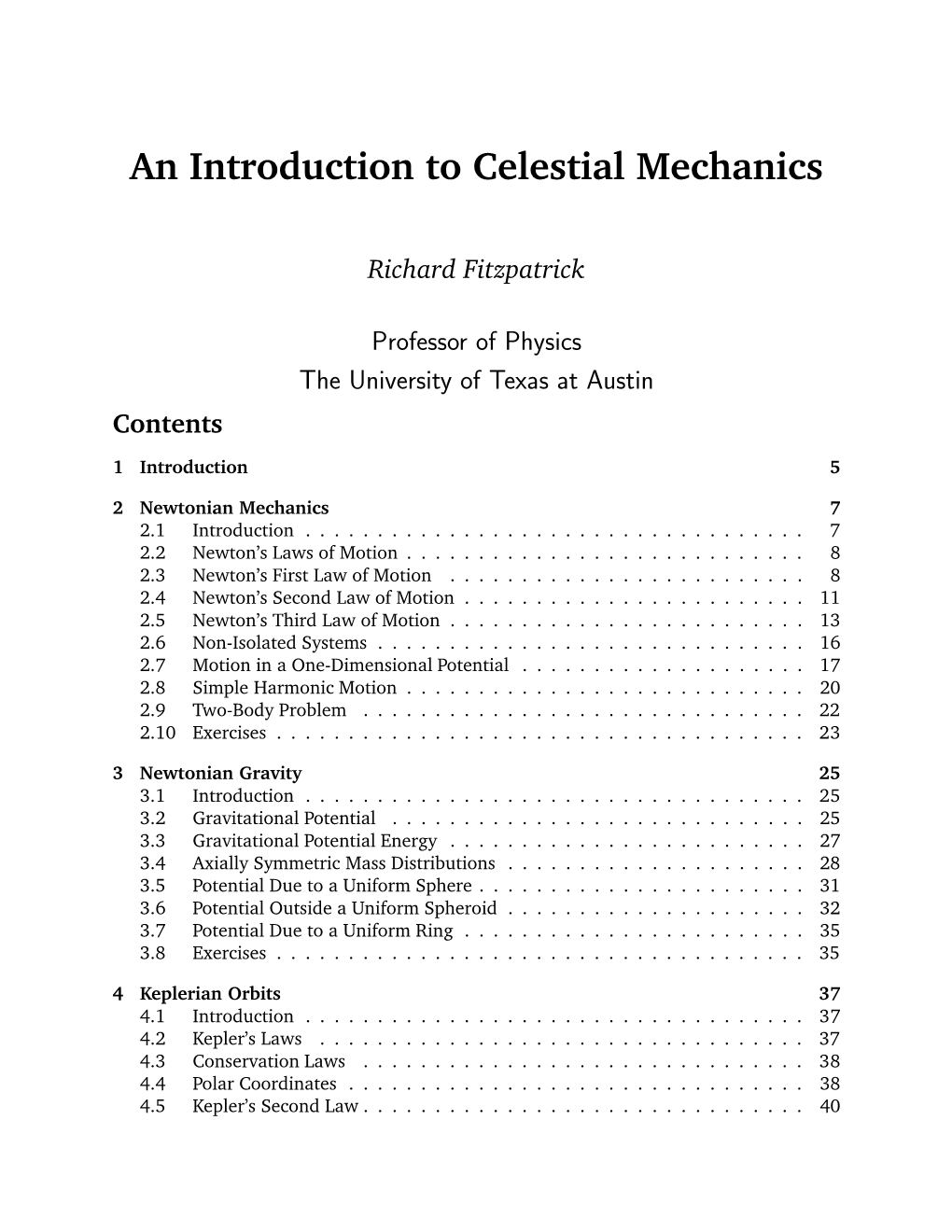
However, this is only true in special frames of reference called inertial frames. Indeed, we can think of Newton’s first law as the definition of an inertial frame: i.e., an inertial frame of reference is one in which a point object subject to zero net external force moves in a straight-line with constant speed. Newtonian Mechanics 9yy′ u t xx′ origin
Figure 2.1: A Galilean coordinate transformation.
Suppose that we have found an inertial frame of reference. Let us set up a Cartesian coordinate system in this frame. The motion of a point object can now be specified by giving its position vector, r ≡ (x, y, z), with respect to the origin of the coordinate system, as a function of time, t. Consider a second frame of reference moving with some constant velocity u with respect to the first frame. Without loss of generality, we can suppose that the Cartesian axes in the second frame are parallel to the corresponding axes in the first frame, that u ≡ (u, 0, 0), and, finally, that the origins of the two frames instantaneously coincide at t = 0—see Figure 2.1. Suppose that the position vector of our point object is r′ ≡ (x′, y′, z′) in the second frame of reference. It is evident, from Figure 2.1, that at any given time, t, the coordinates of the object in the two reference frames satisfy x′ = x − u t, y′ = y,
(2.1)
(2.2)
(2.3) z′ = z.
This coordinate transformation was first discovered by Galileo Galilei, and is known as a Galilean transformation in his honor.
By definition, the instantaneous velocity of the object in our first reference frame is given by v = dr/dt ≡ (dx/dt, dy/dt, dz/dt), with an analogous expression for the velocity, v′, in the second frame. It follows from differentiation of Equations (2.1)–(2.3) with respect to time that the velocity components in the two frames satisfy vx′ = vx − u, vy′ = vy,
(2.4)
(2.5)
(2.6) vz′ = vz.
These equations can be written more succinctly as v′ = v − u.
(2.7) 10 CELESTIAL MECHANICS
Finally, by definition, the instantaneous acceleration of the object in our first reference frame is given by a = dv/dt ≡ (dvx/dt, dvy/dt, dvz/dt), with an analogous expression for the acceleration, a′, in the second frame. It follows from differentiation of Equations (2.4)–
(2.6) with respect to time that the acceleration components in the two frames satisfy ax′ = ax, ay′ = ay, az′ = az.
(2.8)
(2.9)
(2.10)
These equations can be written more succinctly as a′ = a.
(2.11)
According to Equations (2.7) and (2.11), if an object is moving in a straight-line with constant speed in our original inertial frame (i.e., if a = 0) then it also moves in a (different) straight-line with (a different) constant speed in the second frame of reference (i.e., a′ = 0). Hence, we conclude that the second frame of reference is also an inertial frame.
A simple extension of the above argument allows us to conclude that there are an infinite number of different inertial frames moving with constant velocities with respect to one another. Newton throught that one of these inertial frames was special, and defined an absolute standard of rest: i.e., a static object in this frame was in a state of absolute rest. However, Einstein showed that this is not the case. In fact, there is no absolute standard of rest: i.e., all motion is relative—hence, the name “relativity” for Einstein’s theory. Consequently, one inertial frame is just as good as another as far as Newtonian mechanics is concerned.
But, what happens if the second frame of reference accelerates with respect to the first?
In this case, it is not hard to see that Equation (2.11) generalizes to du a′ = a −
,
(2.12) dt where u(t) is the instantaneous velocity of the second frame with respect to the first.
According to the above formula, if an object is moving in a straight-line with constant speed in the first frame (i.e., if a = 0) then it does not move in a straight-line with constant speed in the second frame (i.e., a′ = 0). Hence, if the first frame is an inertial frame then the second is not.
A simple extension of the above argument allows us to conclude that any frame of reference which accelerates with respect to a given inertial frame is not itself an inertial frame.
For most practical purposes, when studying the motions of objects close to the Earth’s surface, a reference frame that is fixed with respect to this surface is approximately inertial.
However, if the trajectory of a projectile within such a frame is measured to high precision then it will be found to deviate slightly from the predictions of Newtonian mechanics—see
Chapter 6. This deviation is due to the fact that the Earth is rotating, and its surface is Newtonian Mechanics 11 therefore accelerating towards its axis of rotation. When studying the motions of objects in orbit around the Earth, a reference frame whose origin is the center of the Earth, and whose coordinate axes are fixed with respect to distant stars, is approximately inertial.
However, if such orbits are measured to extremely high precision then they will again be found to deviate very slightly from the predictions of Newtonian mechanics. In this case, the deviation is due to the Earth’s orbital motion about the Sun. When studying the orbits of the planets in the Solar System, a reference frame whose origin is the center of the Sun, and whose coordinate axes are fixed with respect to distant stars, is approximately inertial.
In this case, any deviations of the orbits from the predictions of Newtonian mechanics due to the orbital motion of the Sun about the galactic center are far too small to be measurable. It should be noted that it is impossible to identify an absolute inertial frame—the best approximation to such a frame would be one in which the cosmic microwave background appears to be (approximately) isotropic. However, for a given dynamical problem, it is always possible to identify an approximate inertial frame. Furthermore, any deviations of such a frame from a true inertial frame can be incorporated into the framework of Newtonian mechanics via the introduction of so-called fictitious forces—see Chapter 6.
2.4 Newton’s Second Law of Motion
Newton’s second law of motion essentially states that if a point object is subject to an external force, f, then its equation of motion is given by dp
= f,
(2.13) dt where the momentum, p, is the product of the object’s inertial mass, m, and its velocity, v.
If m is not a function of time then the above expression reduces to the familiar equation dv m
= f.
(2.14) dt
Note that this equation is only valid in a inertial frame. Clearly, the inertial mass of an object measures its reluctance to deviate from its preferred state of uniform motion in a straight-line (in an inertial frame). Of course, the above equation of motion can only be solved if we have an independent expression for the force, f (i.e., a law of force). Let us suppose that this is the case.
An important corollary of Newton’s second law is that force is a vector quantity. This must be the case, since the law equates force to the product of a scalar (mass) and a vector
(acceleration). Note that acceleration is obviously a vector because it is directly related to displacement, which is the prototype of all vectors—see Appendix A. One consequence of force being a vector is that two forces, f1 and f2, both acting at a given point, have the same effect as a single force, f = f1 + f2, acting at the same point, where the summation is performed according to the laws of vector addition—see Appendix A. Likewise, a single force, f, acting at a given point, has the same effect as two forces, f1 and f2, acting at the 12 CELESTIAL MECHANICS same point, provided that f1 + f2 = f. This method of combining and splitting forces is known as the resolution of forces, and lies at the heart of many calculations in Newtonian mechanics.
Taking the scalar product of Equation (2.14) with the velocity, v, we obtain dv m d(v · v) m dv2
==m v· = f · v.
(2.15) dt 2 dt 2dt
This can be written where dK dt
= f · v.
(2.16)
(2.17)
1
K = m v2.
2
The right-hand side of Equation (2.16) represents the rate at which the force does work on the object (see Section A.6): i.e., the rate at which the force transfers energy to the object.
The quantity K represents the energy that the object possesses by virtue of its motion. This type of energy is generally known as kinetic energy. Thus, Equation (2.16) states that any work done on point object by an external force goes to increase the object’s kinetic energy.
Suppose that, under the action of the force, f, our object moves from point P at time t1 to point Q at time t2. The net change in the object’s kinetic energy is obtained by integrating Equation (2.16):
An Introduction to Celestial Mechanics