Section Five: Analyzing a dataset
In this section we shall use the dataset we created in the second section to show how we perform an analysis of the dataset.
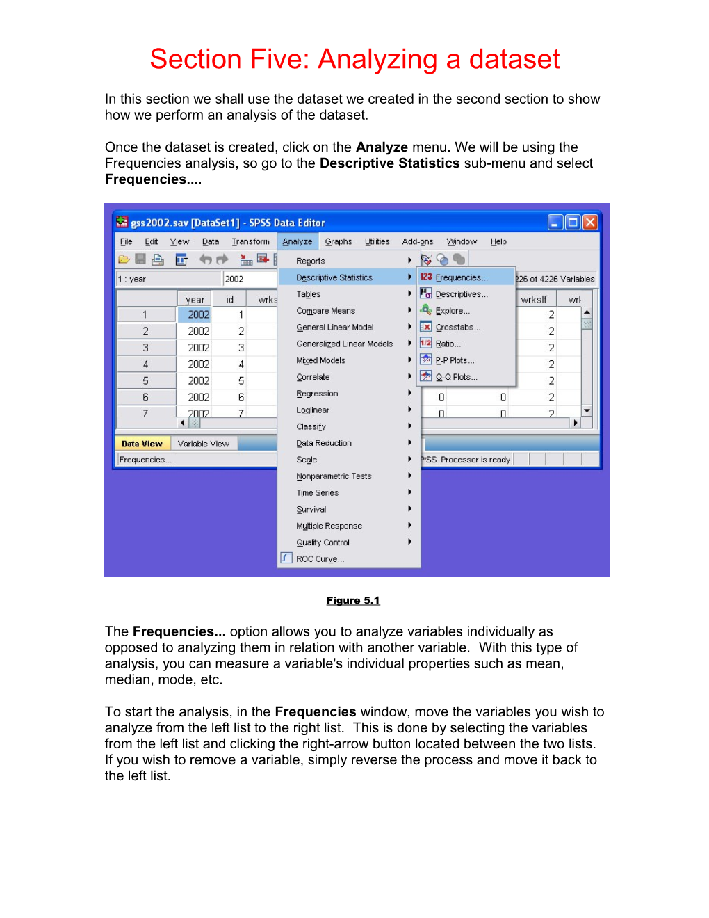
Once the dataset is created, click on the Analyze menu. We will be using the Frequencies analysis, so go to the Descriptive Statistics sub-menu and select Frequencies....
Figure 5.1
The Frequencies... option allows you to analyze variables individually as opposed to analyzing them in relation with another variable. With this type of analysis, you can measure a variable's individual properties such as mean, median, mode, etc.
To start the analysis, in the Frequencies window, move the variables you wish to analyze from the left list to the right list. This is done by selecting the variables from the left list and clicking the right-arrow button located between the two lists. If you wish to remove a variable, simply reverse the process and move it back to the left list.
Figure 5.2
Once you have chosen the required variables and set your display options, click the "OK" button. Another window will open up with the outputs displayed in the following format:
Figure 5.3
You can save this output window by clicking on the "Save" button. You can close this window once the output has been saved.
You can also delete the output, by clicking on the "Output" option in the left window, and then hitting the "Delete" button. If you leave this window open, and run another analysis, then the output for that run will be stacked under the existing output. If you print this output, then all the analysis outputs will be printed, so it is recommended that you delete the output analysis from the output window once you have saved them.
For the rest of this section, you will need to change how the variables are listed in the analysis windows. If you need help, please refer to Section Four: Changing how variables are listed.
Next, we will show you how to display more statistics with your univariant analysis. For this example, we will use the 2002 GSS dataset. For help with opening a GSS dataset, please refer to Section Three: Opening an existing dataset. First, click on the Frequencies tab under the Analyze menu. The following window will open up, where you can choose which variables you want to analyze.
Figure 5.4
In our example we will perform a frequency analysis of the respondent's Zodiac sign (zodiac), age (age), and number of people in their household (hompop).
Figure 5.5
Next, click on the 'Statistics' button at the right of the Frequencies window. Another window will open up where you can decide the type of analysis you want to perform. In figure 5.7, mean, median and mode analyses are performed. Check the boxes next to the statistics you wish to see calculated.
Figure 5.6
Once you click "OK," another output window will open. This window contains a box with the mean, median, and mode of both variables.
Figure 5.7
Now, we will show you how to perform a bivariant analysis on the given data set. Again, this example will use the 2002 GSS dataset. First, under the Analyze menu, select the Crosstabs option in the Descriptive Statistics sub-menu. At the Crosstabs window, we will perform an analysis of "Sex" vs. "Zodiac Sign." Remember, the independent variable goes into the columns box while the dependent variable always goes into the row box.
Figure 5.8
Once you have clicked "OK," an output window will display a statistical breakdown of the "Sex" variable in its relation to the "Zodiac" variable.
Figure 5.9
You can also change the cell display from the Crosstabs window. In the window, click the "Cell Display" button. This displays the Crosstabs: Cell Display window. From there, you can choose from many different display options.
Figure 5.10
One of the most commonly used options is the "Chi-Square" option, which can be enabled by clicking the "Statistics" button in the Crosstabs window. Then, check the "Chi-Square" checkbox, click "Continue," then "OK."
Figure 5.11
Figure 5.12 shows how the Chi-Square is displayed in the Output window.
Figure 5.12
Section Five: Analyzing a Dataset
