Geophysics 224
Lab 3 : Ray tracing and shot gathers
Introduction
Reflection seismic methods are the most widely used exploration tool in hydrocarbon exploration. Profiles can be as long as some hundred kilometers while 3D seismic projects usually cover areas of some hundreds of square kilometers.
In 2D, the receiver (geophones) and sources (dynamite or vibroseis) are usually aligned. The reflected energy is recorded by geophones and displayed as common shot gathers. Geophones close to the source receive the signal first. Usually, but not always, the reflected energy can be recognized for their hyperbolic shape.
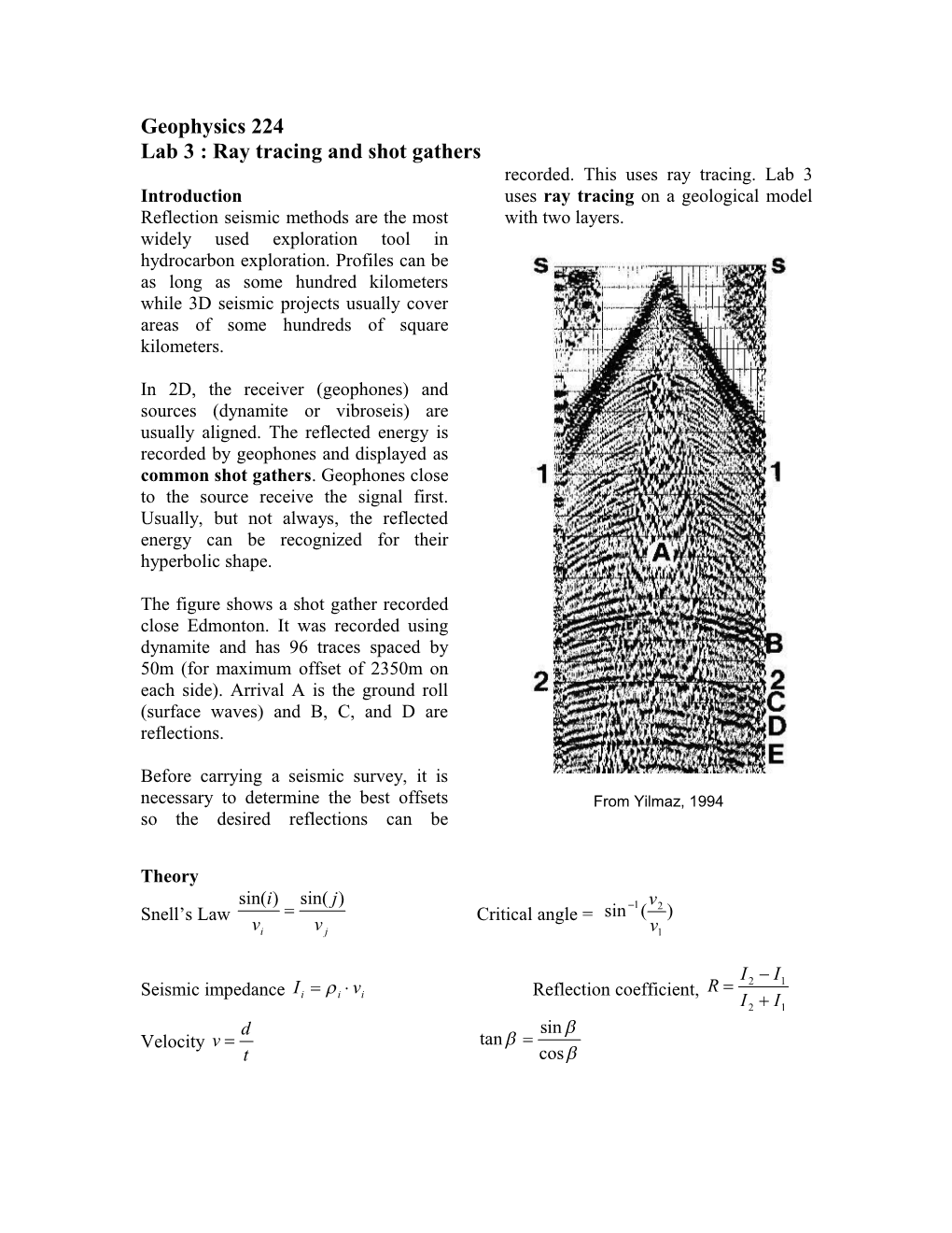
The figure shows a shot gather recorded close Edmonton. It was recorded using dynamite and has 96 traces spaced by 50m (for maximum offset of 2350m on each side). Arrival A is the ground roll (surface waves) and B, C, and D are reflections.
Before carrying a seismic survey, it is necessary to determine the best offsets so the desired reflections can be recorded. This uses ray tracing. Lab 3 uses ray tracing on a geological model with two layers.
From Yilmaz, 1994
Theory
Snell’s Law Critical angle =
Seismic impedance Reflection coefficient,
Velocity
Ray tracing
We will ray trace for the model shown below:
The density and velocity are known from logs on well close this area
Sandstone / Limestone / DolomiteDensity (g/cc) / 2.2 / 2.7 / 2.6
Wave velocity (m/s) / 2500 / 4500 / 4000
Part – 1
Ray tracing will show which rays will arrive at the geophones located every 100m for a split spread array (geophones located on both sides of the source). The distance between the source and the first geophone is 100m and the maximum offset is 4100 m.
First compute the angle of incidence of the rays that will reach each geophone (100m, 200m,.…). To do this, use the Excel spreadsheet.
(1) Guess a value for the angle of incidence (take-off angle)
(2) Look at the offset at which the ray returns to the surface
(3) If the offset is too large, decrease the angle and vice versa
(4) Continue until your offset is within + 1m of the geophone
(5) Repeat the same procedure for all geophone on both sides of the array.
Plot (in Excel) both reflections as a shot gather. This will be a plot of travel time versus distance.
Part – 2
Trace the rays that will reach the geophones located at 500, 1000, 2000 and 3000 m offset on both sides for both reflections.
Part – 3
Suppose the wave amplitude at the source was 1. Ignore amplitude decay effects (geometrical spreading, attenuation, etc) and calculate the expected amplitudes for both reflections (assuming normal incidence).
Now sketch/plot the same shot gather with traces located at 500,1000,2000,3000 and 4000m with the relative expected amplitudes.
Questions
1.Do the reflections intercept each other? Why?
2.What are the relative sizes of first and second reflection? How can we explain this effect?
3.How different would a real shot gather appear? What other events can we expect? Explain.